Sample Calculation:
For radius of 0.53 m
Period of One cycle = Period of 10 cycles / 10
T = 8.19/10
T = 0.819 s
The same process was utilised to figure out the period for one oscillation for each other independent variable.
Controlled Variables:
(Note: These masses were also measured in grams; however converting it to SI units is more productive.)
Data table #2: Manipulating Spinning mass (ms)
Controlled Variables:
Data Table # 3: Manipulating Hanging Mass (Mh)
(Note: The formula expressed has previously been derived such that F is equivalent to the Weight of the hanging mass. Thus, it is beneficial to create a graph between Mh rather than F itself which compiles of Mh times the accepted value of acceleration due to gravity, only indirectly describing the relation between Mh and f.)
Controlled Variables:
(Note: The uncertainty on each of the Period is an estimated guess. An electronic stopwatch was used which has a precision of uptil 0.01 s. Assuming that the reaction time was perfect, we get a manufacturer’s uncertainty of 0.01 s. However, the idea of reaction time will be explained later on in the Section of Evaluation).
The most important qualitative observation recorded was the idea of the radius of the circular movement, not being the length of the string. Due to disequilibrium of the force exerted for the motion to occur, the actual radius would form a Pythagorean relationship with the length of the string as the length becomes the hypotenuse and this relationship will be explained later on in the Evaluation section.
Manipulated Data
The Manipulated Data section (not to be confused with previous manipulating radius and mass etc) will include all the data calculated with respect to the data collected from the actual experiment. Here it will be convenient to use the converted raw data for legitimate results. A data table for frequency and frequency2 will be shown with respect to the independent variables.
Data Table #4: Frequency for Manipulating Radius
(Remember; , and the uncertainty for T propagates for the uncertainty of f as shown later on in the calculations)
Sample Calculation for frequency (uncertainty)
For radius = 0.53 m;
T1 = 0.819 s (+/- 0.001s)
(Convert to relative uncertainty)
Data table # 5: Frequency2 for (1/r) [with respect to the formula attained]
Sample Calculation for (1/R):
Radius: 0.53 m
=
= Relative Uncertainty
= Absolute Uncertainty
Sample Calculation for f2:
Radius: 0.53m; Frequency: 1.22 0.001 Hz
F2 = 2
F2 = Relative Error
F2 = Absolute Error
This process was followed to attain the correct uncertainty and the actual value for each of the values represented in the data above. For the following tables, which require the reciprocal of the original independent value, the same method was use (for e.g. 1/ms) and the same method was applied to figure out the f2 value.
Data Table # 6: Frequency for Manipulating Spinning Mass (ms)
Data Table # 7: Frequency2 for Manipulating (1/ms)
This equation was derived from the previous equation provided, and helps us determine the relationship between Ms and frequency in a linear manner. A further graphical explanation will be provided in the Graphical Analysis part.
Data Table # 8: Frequency for Manipulating Hanging Mass (Mh)
Data Table # 9: Frequency2 for Manipulating Hanging Mass (Mh)
This equation has also been derived from the original equation provided. It provides a linear relationship between the hanging mass and f^2 which will be further discussed in the graphical analysis section.
Graphical Analysis
(Notice that due to the precision of the data and its closeness, an average of the trials was taken by the graphing program. By visualizing the data, we see that it is very precise, and its accuracy will be measured later on in this section of graphical analysis. The scatter plot is an average of the two trials which leads to more precise and accurate answers, and eliminates any random errors.)
- Manipulating Radius
This section describes the basic relation between Frequency and radius, as well as the manipulated relation between Frequency2 and 1/r, which is attained from the formula provided. As visible from the graph of Frequency vs. Radius, an indirectly proportional relationship is visible and thus the line of best fit provided for that graph is a rational function. As radius increases, frequency decreases. This is due to the fact that when the radius of a circle motion increases, if the mass of an object and the hanging mass are kept constant, the object must travel a longer distance around the circle, since increasing the radius means increasing the circumference of the circular path taken. The frequency, as a result, decreases.
However, a linear graph is then attained from using the formula;. The graph is a straight line because f2 is indirectly proportional to r. The original formula does not have any y intercept, however for the equation gained from the graph above there is a definite y intercept or b value. This is due to a systematic error. The R^2 value is close to 1 which means that the random error is eliminated and this is done through averaging. The actual slope gained from plugging in the controlled/constant values for this experiment is:
Slope = ; where the accepted value of g is assumed to be 10ms-2.
Slope = ; (relative)
Slope = 0.6061 ± 0.0004 Hz2r (absolute)
We can see that there is a definite error in this experiment from the comparison of the slopes and the percentage error will be measured in the conclusion.
- Manipulating Spinning Mass
This section describes the relationship between frequency and the mass of the spinning object. A graph is also created like the previous section, from the manipulated equation. From the Frequency vs. spinning mass graph, one can visualize that frequency is indirectly proportional to frequency. A straight line graph is then provided from the manipulated equation of, where
This relationship is explanatory without an equation. If the radius of a horizontal circular motion is kept constant and the force is kept constant correspondingly, the mass is inversely proportional to the frequency. If mass increases, it is difficult for that amount of force to push the mass around a circle, and thus reducing the frequency.
The graph created from the manipulated equation also has a y intercept; which means that it is subject to a systematic error. However, the precision for both graphs is close to perfect, as R2 value almost approaches 1. The theoretical slope will be determined in this section and will later be utilised in the conclusion section to find the percent error.
Slope =
Slope = (relative)
Slope = 0.0491 ± 0.0006 Hz2m (absolute)
The theoretical slope is also different by a bit, showing that there is a high percent error which will be evaluated in the conclusion.
- Manipulating Hanging Mass
This section represents the relationship between frequency and the hanging mass (which, when manipulated, provides a change in the force of the system). A graph of f2 vs. m (h) is then created to provide a linear representation of this relationship. As we can reflect from the first graph, the relationship between frequency and hanging mass is directly proportional. If the force in the tension is increased, keeping the radius and the spinning mass constant, this will mean that the extra force will help the motion of the object and decrease the time period, thus increase frequency. The R2 value is very close to 1 which means the data is precise for both the graphs. From the equation provided we have also extrapolated:
; which means that. The theoretical slope can we figured out as we know the values of the constant;
m =
m = (total relative error)
m = 35.254 ±0.059 Hz2kg-1 (total absolute error)
Therefore, we can thus conclude that there was yet again a high amount of uncertainty and it will be calculated through the percent error. The systematic error still exists, however random errors are not as frequent in this experiment.
Conclusion
The graphical analysis states all the basic trends attained from the graph. The following trends will be re-evaluated in this section, as well as the percent error will be calculated to describe the inaccuracy of the values.
The trend for manipulating the radius of the circular motion is that as the radius increases, the frequency decreases, resulting in an inversely proportional relation between the two. The percentage error calculation can be made by utilising the slope of the line and the theoretical slope (since the variables kept constant result in a theoretical value of the slope).
Radius: Theoretical slope = 0.6061; Experimental slope = 0.8392
(Absolute Value)
This is a relatively high error (neglecting uncertainties). The error can be due to the fact that the length of the string was not always the radius of the circular motion; if not enough force was exerted the string will make a Pythagorean relationship, with horizontal and vertical components, where the horizontal component is the actual radius of the circle. Other error sources will be discussed in the evaluation. The equation of our line also has a y intercept; y = 0.8392x - 0.0311; where - 0.0311 is the y intercept. This means that if the radius was 0, the frequency will be – 0.0311, which absolutely makes no sense since frequency cannot be negative. And a radius of 0 m means no motion can occur, therefore (0,0) could have been included as a point; although not measured. The y intercept also suggests that the values for the frequencies will be more than the theoretical.
The trend for manipulating the spinning mass is also inversely proportional to the frequency of that motion. As the mass increases, the general frequency will decrease. The following suggests the percentage error for the spinning mass experiment:
Spinning Mass: Theoretical slope = 0.0667; Experimental slope = 0.0491
This is also a relatively intense error. The sources of error can be the unadjustable radius, as it was not constant as proven by the Pythagorean relation, and the human force that is exerted might be uneven.
The trend for hanging mass (force) and the frequency of a circulation motion is, unlike the other two factors, directly proportional. This makes sense, since having more tension in the string leads to a quicker speed, thus an increase in the frequency. The percent error for this is calculated below:
Hanging Mass: Theoretical slope = 35.254; Experimental slope = 36.368
(Absolute Value)
This error is really small compared to the rest; this can be due to the fact that there are no real factors that affect the force of the tension. The only source of error can be the human force applied to sustain motion.
Evaluation (Sources/Solutions of error)
This section deals with the sources of error, and the improvements that one can utilise to improve this experiment.
The first two major sources of error are quite evident. The major source of error as described in previous sections is the fact that the length of the string is not the same as the radius of the horizontal circular motion. This is described further in this section. The diagram illustrates how the motion looked like when a little bit of force applied, was taken away to let the tension in the string take over the motion. That was not possible due to the slightest of air resistance. The horizontal component labelled as r would be known as the radius since the mass spins at an angle from the horizontal. This however is hard to measure and thus is assumed to be constant.
The second major source of error is the reaction time. The fact that only two trials were taken, it is not enough to eliminate the idea of a random error. This is because a change in reaction time may occur. Reaction time is neglected throughout this experiment, and assumed to be perfect. This is why only the manufacturer’s uncertainty was taken for the stopwatch. Since it is a digital device, the smallest unit is the uncertainty. However, reaction time was a major factor and the idea of a bad reaction time could not be eliminated by taking more trials. Although, an attempt to keep it unimportant was made by having the same person and their frame of reference decide, when to start and when to stop.
Some non-major sources of error could be those such as air resistance. Although, not much air was there, but the air molecules do interfere with the radius going down at an angle, and more human force being required for the system compared to the force originally caused by the Hanging mass.
These errors lead to a systematic error, and the y-intercepts in each manipulated equation reflects that. The experiment could be made better in a sense that, more trials are taken for each different sub-experiment. The person revolving can also make sure that they put enough force behind it to overcome the force of resistance. Also a constant speed would be required for more accurate results. The manipulated graphs could have also had a line of best fit, which touched 0 in order to get a more accurate slope, since there were no y intercepts in the original equation. But if the data was accurate, then the line would have automatically touched 0.
All in all, the percent error can be high due to the fact that we deal with quite small numbers. This experiment does consist of some systematic errors which can be improved on.
Instruction # 4
Finding the mass of a rubber stopper
Radius = 0.53 (+/- 0.0005m)
Frequency = 1.22 (+/- 0.001 Hz)
Hanging mass = 0.03237±0.00001 kg
The original spinning mass of the stopper is 0.013 kg.
This means that the error is really low, and that this value is valid.