5 Coefficient of Static Friction. (n.d.). Byju’s. https://byjus.com/physics/coefficient-of-static-friction/ 6Kognity. (n.d.). B.1.1 Torque.
https://app.kognity.com/?next=/study/app/physics-hl-2016/engineering-physics/b1-rigid-bodies-a nd-rotational-dynamics/torque/
moment of inertia7 ( I ) = mass (m)×radius2(r2 ) and angular acceleration8 ( α) = linear acceleration (a)
Now Iα = F
static
r can be rewritten as: (m×r2 )
× a = F
static r
which can be simplified to:
F static
= (m×a) (Equation 4)
Having obtained frictional force in equation 4, it can now be used to calculate
acceleration using equation 3:
ma = mg sinθ
(m×a)
2
Collecting like terms gives:
mg sinθ
3 ma 2
Rearranging for acceleration:
a = 2 g sinθ (Equation 5)
Equation 5 can now be used to obtain velocity using the equation for uniform translational motion: v2 = u2 + 2as . Noting that the car moves from rest in this experiment, initial velocity ( u )
is zero, thus:
v2 = 2as . Acceleration can be substituted using equation 5 to give:
v2 = 4 gsinθ s
which can be solved for velocity:
v = √
4 gsinθ
3
(Equation 6)
Hypothesis
It can be postulated that the velocity will be highest on wood since it appears to be the smoothest object, hence having the lowest coefficient of friction produces a smaller frictional force allowing for converting more potential energy to kinetic energy. A higher kinetic energy at
7 Kognity. (n.d.-b). B.1.3 Moment of Inertia.
https://app.kognity.com/?next=/study/app/physics-hl-2016/engineering-physics/b1-rigid-bodies-a nd-rotational-dynamics/moment-of-inertia/
8 Kognity. (n.d.-c). B.1.4 Uniform Angular Acceleration.
https://app.kognity.com/?next=/study/app/physics-hl-2016/engineering-physics/b1-rigid-bodies-a nd-rotational-dynamics/uniform-angular-acceleration/
the bottom of the incline means the car is travelling at a higher velocity. It can further be hypothesised that the plane with the highest angle of inclination will result in the highest velocity for the car based on the knowledge that higher incline produces larger acceleration.
Variables
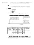
Independent: Coefficient of static friction, Angle of inclination of plane
The coefficient of static friction is different for each material; this investigation evaluates how the coefficient of static friction on three surfaces (wood, cardboard, rubber) and angle of inclination (10, 20, 30, 40, 50, 60, 70, 80 º ) plane influences the velocity of a model car rolling
down an incline plane.
Dependent: Velocity of model car
This research investigates the effects of varying the independent variables on the velocity of a model car, where velocity can be calculated dividing the displacement by the time taken.
Controlled: Table 1: Identifying and analysing controlled variables
Methodology
In order to answer the research question, the methodology for this investigation entails an experiment. This investigation will use planes made of three materials: rubber, cardboard, and wood. The planes will then be inclined at eight different angles: 10, 20, 30, 40, 50, 60, 70, and
80 degrees.
The coefficient of static friction ( μ ) for each plane will be measured by 3 trials of the
angle at which the car starts rolling; and is calculated using equation 2, where θ is the angle of
inclination of the plane at which the car starts rolling:
μ = tanθ (From equation 2)
Time taken for the car to traverse the plane will be measured doing 5 trials at each angle of incline for each material, the value will be obtained using the video analysis software Camtasia 39. Since the values are in close proximity they will be taken to 5 decimal places. The velocity of the car while traversing the plane and can then be determined using equation 7:
velocity of the car (ms1) = length of plane (m) (Equation 7)
In order to investigate and quantify a relationship between θ , μ , and velocity, data from
the experiment needs to undergo statistical tests. Given that this investigation involves continuous predictor and outcome variables, the data will be analysed with correlation and regression analysis10 to investigate relationships and intensity of the correlation11. This will
9 Camtasia 3. (2002). [Video Editing Software]. TechSmith.
.html
10 Leeper, J. (n.d.). Choosing the Correct Statistical Test in SAS, Stata, SPSS and R. UCLA Institute for Digital Research & Education. https://stats.idre.ucla.edu/other/mult-pkg/whatstat/ 11 UT Austin. (n.d.). Pearson Correlation and Linear Regression.
%20analysis%20provides%20information,variable%20based%20on%20the%20other.
involve use of the Graphic Display Calculator (GDC), to obtain values for Pearson’s correlation coefficient ( r ) and the coefficient of determination ( R2 ) which can then be used to determine
the fit of the regression line to the data.
Although other methods that can be employed to find velocity, this approach was chosen for its low uncertainty and high precision. Furthermore, the pandemic limited my access to equipment hence enforcing my choice of this methodology. Adopting alternative approaches with complete tools would yield more precise results; nonetheless I have considered the limitations of this approach later in this investigation.
Materials
Table 2: Listing Apparatus and Materials
Safety, Ethical, & Environmental considerations
No ethical or environmental issues were found, and no safety hazards were found.
Procedure
A: Finding the velocity for each incline
The wood plane was aligned with the 10 º marking on the protractor, and rested against
the clamp and stand, the camera was deployed to capture the length of the plane. The recording was started and car rolled down the incline, this was repeated four times for this angle, and subsequently repeated five times for angles 20, 30, 40, 50, 60, 70, and 80 º . The plane was then
substituted for cardboard and subsequently the yoga mat. This is depicted in Diagram 3 below, while the image is provided in Appendix 5:
Diagram 3: Experimental setup to find the velocity for each incline
B: Finding coefficient of static friction
The wooden plane was held parallel to the floor, adjacent to the protractor. The car was placed on the plane, and the plane slowly tilted until the car started moving, the angle when the car started moving was noted and this step was repeated twice. The wood was then substituted by cardboard sheet. Finally, the cardboard was replaced by the yoga mat. This is depicted in Diagram 4 below:
Diagram 4: Experimental setup to find the coefficient of static friction for each material
Data and Analysis
- Experimental data
The data gathered through procedures A and B is presented below; the uncertainty in time originates from the discrepancy of 1 frame in 30 fps footage, while uncertainty in angle comes from uncertainty in the protractor. The complete data tables can be found in the appendix.
Table 3: Raw data of materials, inclines and time taken by car (Appendix 1)
Table 4: Raw data of materials and angle at which model car starts rolling (Appendix 2)
Data Processing and Uncertainty Propagation
Table 5: Data of materials, inclines and velocity (Appendix 3)
Example calculation of velocity:
Example velocity for Cardboard at 30º trial 4
Table 6: Data of materials and coefficient of static friction
Example calculation of coefficient of static friction: Example for Wood trial 2
Table 7: Data of coefficient of static friction and velocity
Data Analysis
The processed data for velocity as a function of angle of incline indicates positive correlation, which is seen in figure 1 below:
Figure 1: Graphing the relationship between velocity and incline (using data in Table 4)
ms1
The highest velocity is observed at the 80 degrees incline, which for wood was 1.754 The trend in figure 1 can be quantified by the correlation coefficient ( r ): 0.981 for wood,
0.993 for cardboard, and 0.981 for rubber. And the values of R2 which are: 0.963, 0.957, and
0.979 for wood, cardboard, and rubber, show the degree of variation in the velocity in relation to
change in incline, these values are very close to 1 indicating strong correlation. This helps answer part of the research question that incline has a positive correlation with velocity, thus increasing it results in higher velocities of the car.
Creating a linear trendline for each curve yielded a non-zero velocity at an incline of
0º , which is incorrect as Newton’s first law of motion states that a body at rest will remain
at rest unless acted upon by an external force, any non zero incline does not result in motion since the weight of the car parallel to the plane cannot overcome the force of static friction. hence logarithmic trend-lines were drawn as they reflect such behavior. Furthermore, based on knowledge from Mathematics Analysis and Approaches topic 2.9 on exponential models, the nature of these curves in this context is appropriate since logarithms depict a rapid rise
in data and subsequent saturation, which is observed12. This behavior when θ approaches
90º
is explained as the plane approaches vertical which means the traction between the wheels
and the surface is overcome by acceleration due to gravity causing the car to free fall as opposed to rolling down the plane, hence resulting in a relatively stable velocity for θ ≥ 90º as the car free
falls.
The relationship between inclination and velocity can be explained referring to two factors, starting with the vector nature of forces. The normal reaction acts perpendicular to the plane, thus the car’s weight is distributed into its perpendicular constituents on an inclined plane in order to balance the forces, it can now be seen that forces parallel to the plane will be = Fsinθ
, and the force perpendicular to F sinθ is equal to Fsin(90 θ) or F cosθ . Applying knowledge
about the increasing nature of the sine function with increasing θ from 0-90, it is apparent that
12 Kognity. (n.d.-d). 2.9.3 Logarithmic Functions.
https://app.kognity.com/?next=/study/app/ibdp-mathematics-analysis-and-approaches-hl/function s/exponential-functions/logarithmic-functions/
larger inclines result in greater force which is proportional to acceleration according to Newton’s second law13. Using the equation for translational motion ( v2 = 2as ) acceleration ( a ) is
proportional to v2 , hence a larger θ results in a greater velocity.
Another explanation for the results can be offered referring to trigonometric relationships and the law of conservation of energy, The angle of incline ( θ ) is an angle of elevation, thus
higher values of ( θ ) with a fixed horizontal distance of lead to an increase in height. As height
increases gravity does more work to exert a greater amount of potential energy on the car since potential energy is proportional to height. Due to the law of conservation of energy, greater potential energy for larger inclines is converted to greater kinetic energy thus larger velocity for the car from higher inclines. Both of these factors theoretically suggest a positive correlation between the variables, which has been observed.
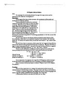
In order to evaluate the reliability of the data, a theoretical approach to determine velocity must be undertaken. Noting the law of conservation of energy and formulas for kinetic and
potential energy gives the following equation: 1 mv2 = mgh
Rearranging for v
gives:
v = √2gh (Equation 8)
Where g is acceleration due to gravity and h is height. Using equation 8 and trigonometric ratios
to determine the height and velocity of the car results as follows:
13 Kognity. (n.d.-e). 2.2.4 Forces and Interactions. https://app.kognity.com/?next=/study/app/physics-hl-2016/mechanics/forces/forces-interactions/
Table 8: Data of theoretical average velocity (using equation 8)
Example calculation of average velocity for inclines: Example average velocity for 30º
It is apparent a large discrepancy exists between values in table 8 and the experimental results. The data in table 8 is only reliable if the entire system consists of only the car and the earth without any restrictive forces, since this is not true, a large discrepancy exists. In order to account for this, the conservation of energy in rotational dynamics can be considered. The kinetic
energy of a rotating body is given by:
E = 1 Iω2 but since the body itself is also in motion, the
formula becomes:
E = 1 Iω2 + 1 mv2
Setting this equal to potential energy and solving for
2 2
velocity gives:
1 Iω2 + 1 mv2 = mgh Where I = m×r2 and ω = v thus giving: v2 + v2 = gh
2 2 2 r 4 2
3 2
4
= gh
v = √ 4 gh (Equation 9)
It is apparent that velocity yielded by this formula will be less than the value determined
using equation 8 ( v = √2gh ). Equation 9 is equivalent to equation 6 ( v =
√4 gsinθ s ) since sinθs
is equal to the height. Using equation 9 to determine the velocity of the car results as follows:
Table 9: Data of theoretical average velocity (using equation 9)
Example calculation of average velocity for inclines: Example average velocity for 30º
The values in table 9 are inaccurate as they do not involve air resistance, and the fact that mass is not equally distributed over the circumference of a wheel. The distribution of mass is relevant because moment of inertia is given by the sum of the product of the mass and the square
of the radius for every point on the circumference of the wheel14 (I = Σ m (r )2 ). In calculating
moment of inertia it is assumed that mass is uniformly distributed, because determining the mass at every instant at every point on the wheel is unattainable; this reduces the accuracy of the results. Nonetheless, these values can still be considered for evaluating the experimental results in the context of this investigation.
14 Kognity. (n.d.-b). B.1.3 Moment of Inertia.
https://app.kognity.com/?next=/study/app/physics-hl-2016/engineering-physics/b1-rigid-bodies-a nd-rotational-dynamics/moment-of-inertia/
Table 10: Data of theoretical vs experimental average velocity
Example calculation of percentage error in velocity: Example average velocity for 30º
These values are sizable but accounting for limitations of both the theoretical calculations and experimental tools, these values are justified. They suggest a systematic error in the results, which will be further discussed in the conclusion and evaluation.
The data in table 6 shows a negative correlation between velocity of the car and the coefficient of static friction, as seen in figure 2 below:
Figure 2: Graphing the relationship between average velocity and coefficient of static friction (using data in Table 7)
It was observed that rubber with the greatest μ of 0.2126, produced the lowest average
velocity of 1.164 ms1 . The curve in figure 2 yields r
suggest a moderate negative correlation, while the
value of -0.690. And the R2 : 0.476. These
R2 value suggests that there is significant
variance between the experimental values and the trendline. This variance is likely due to the large absolute uncertainty of the protractor. The relationship in figure 2 can be attributed to frictional forces acting on the car on each surface. The frictional force acts parallel to the incline but in the opposite direction to the thrust force, given that the car moves from rest the weight of the car acting parallel to the plane drives it forward. Since forces are vector quantities, the thrust on the car is the resultant of the difference between weight and friction. The resultant force on
the car decreases on surfaces with a higher value of
μ since
μ is proportional to the frictional
force, while weight remains constant. Noting Newton’s second law,
FNet = ma 15, a smaller net force will lead to less acceleration as the mass of the car remains
constant. With a smaller acceleration the final velocity will be lower as denoted by the adapted
equation for translational motion: v2 = 2as where a∝v2 , hence a lower acceleration will result in
lower final velocity on a plane of constant length.
Evaluating the data analysis, it can be claimed that the measurement uncertainty had
minimal impact on data for θ and velocity since the largest measurement uncertainty in velocity
wass 16.73%. Nevertheless, measurement uncertainty in μ of up to 33.33% may have an impact
on the results, but is not large enough to undermine or require alterations to the analysis. This will be further discussed in the evaluation.
Conclusion and Evaluation
- Conclusion
The data gathered in this investigation suggests that there is a positive relationship between incline and resultant velocity, as seen with correlation coefficients 0.981 for wood, 0.993 for cardboard, and 0.981 for rubber. Similarly, the data suggests that a higher value of μ
leads to lower velocity as shown by the r value of -0.690, suggesting a moderate negative
correlation. These observations allow for a conclusion to this investigation by answering the research question: How do angle of incline and the coefficient of static friction of different surfaces like wood, cardboard and rubber affect the velocity of a wheeled object rolling down an inclined plane? In that an increase in incline angle ( θ ) leads to an increase in
velocity due to the vector nature of forces and the law of conservation energy while the
15 Kognity. (n.d.-e). 2.2.4 Forces and Interactions. https://app.kognity.com/?next=/study/app/physics-hl-2016/mechanics/forces/forces-interactions/
opposite is true for increasing values of μ due to larger frictional forces and Newton’s
second law as more friction results in lower net thrust and hence lower velocity. It was also
observed that the highest velocity (1.754 ms1 ) was achieved with the largest value of θ
(80º) and on the material with the smallest μ (wood). These results support the hypothesis
made earlier in this report as to how the car would have the highest velocity on the wooden surface, and the largest angle will result in greatest velocity.
The results obtained in the investigation are significant because of the vast scale of cars and roads in our daily lives, application of knowledge about the coefficient of friction of materials can significantly impact our ability to combat climate change and increase road safety, as we design more efficient tyres and roads to limit greenhouse gas emissions and reduce accidents, this can also be more cost efficient for individuals who can analyse whether it is worth to pay for more expensive tyres in turn for the higher vehicle efficiency.
Evaluation
The results obtained in this investigation can be considered reliable as the percentage random error for velocity was below 17%, this originates from the absolute uncertainty of the ruler and the footage which was used to measure time; this error has limited impact on the results as it is not very large and 5 trials were conducted to mitigate the impacts. Nevertheless, the
percentage random error in μ was upto 33.33% due to the absolute uncertainty of the protractor,
this high percentage error hinders reliability of the results, however the concordant results of angles on wood and cardboard (Appendix 2) ensure the results are reliable. Additionally, comparing the findings of this investigation to established research shows similar relationships
between incline and velocity16, hence further indicating the reliability and validity of the data in this investigation.
The percentage error in velocity should not be viewed as certain since the theoretical value lacked parameters in the moment of inertia which induce limitations and create a systematic error, hence furthering theoretical values from the experimental hence inflating the percentage error. Although these systematic errors bring the values further from the literature values, the results are still applicable since the trends observed are from results which were all affected in an identical manner by the systematic error. It can be confirmed that this error is systematic as the percent error is significantly higher than the percentage uncertainty.
Beyond this limitation, the strengths of the investigation are presented on the next page:
Table 11: Strengths of the experiment
16 UK Essays. (n.d.). Factors Affecting Velocity of a Sphere Rolling Down Incline. UKEssays.Com.
Although I have pursued this exploration to the best extent of resources available to me, unfortunately there still have been some limitations which are on the next page:
Table 12: Limitations of the experiment
Although there were some limitations this investigation has successfully fulfilled its intent, and could be expanded upon in the following areas for future research:
The study can be redesigned to include a wider variety of surfaces and inclines to get a more accurate trendline of the relationship between the variables, while involving calculations of air resistance as a resistive force to get more accurate theoretical values for evaluation. The
redesigned study should use more precise equipment as identified in the limitations alongside a wider variety of secondary sources such as journals beyond the Physics textbook.
Works Cited
Camtasia 3. (2002). [Video Editing Software]. TechSmith. .html
Coefficient of Static Friction. (n.d.). Byju’s. https://byjus.com/physics/coefficient-of-static-friction/
Khan Academy. (n.d.). Mass on an inclined plane [Illustration]. https://cdn.kastatic.org/ka-perseus-images/e84aaabdfbbaf89b12c74e3ac6f17708b 6ebcaad.png
Kognity. (n.d.-a). B.1.1 Torque.
https://app.kognity.com/?next=/study/app/physics-hl-2016/engineering-physics/b1
-rigid-bodies-and-rotational-dynamics/torque/
Kognity. (n.d.-b). B.1.3 Moment of Inertia. https://app.kognity.com/?next=/study/app/physics-hl-2016/engineering-physics/b1
-rigid-bodies-and-rotational-dynamics/moment-of-inertia/
Kognity. (n.d.-c). B.1.4 Uniform Angular Acceleration. https://app.kognity.com/?next=/study/app/physics-hl-2016/engineering-physics/b1
-rigid-bodies-and-rotational-dynamics/uniform-angular-acceleration/
Kognity. (n.d.-d). 2.9.3 Logarithmic Functions. https://app.kognity.com/?next=/study/app/ibdp-mathematics-analysis-and-approac hes-hl/functions/exponential-functions/logarithmic-functions/
Kognity. (n.d.-e). 2.2.4 Forces and Interactions. https://app.kognity.com/?next=/study/app/physics-hl-2016/mechanics/forces/force s-interactions/
Leeper, J. (n.d.). Choosing the Correct Statistical Test in SAS, Stata, SPSS and R. UCLA Institute for Digital Research & Education.
https://stats.idre.ucla.edu/other/mult-pkg/whatstat/
Physics World. (n.d.). Forces on an inclined plane [Illustration].
Static & Kinetic Friction. (n.d.). David Newman’s Page - University of Alaska Fairbanks. iction.htm
The Editors of Encyclopaedia Britannica. (n.d.). Newton’s laws of motion | Definition, Examples, & History. Encyclopedia Britannica.
UK Essays. (n.d.). Factors Affecting Velocity of a Sphere Rolling Down Incline.
UKEssays.Com.
g-9299.php
UT Austin. (n.d.). Pearson Correlation and Linear Regression.
%20correlation%20analysis%20provides%20information,variable%20based%20o n%20the%20other.
Appendices
Appendix 1: Raw experimental data of materials, inclines and time taken by car
Appendix 2: Raw data of materials and angle at which model car starts rolling
Appendix 3: Data of materials, incline and velocity
Appendix 4: Data of materials and coefficient of static friction
Appendix 5: Image of experimental setup depicted in Diagram 3
Acknowledgements
I would like to thank my extended essay supervisor, Mr Amit Badola for teaching me during the IBDP Physics course and his extensive support during the extended essay process.