Investigating the Oscillations of an Obstructed Pendulum

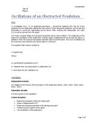
Diagram:

*Figure not drawn to scale

Method:

1. Place the stand on a stable surface, and arrange it like shown on the above diagram.
2. Measure 40cm from the top of the stand to the obstruction and adjust them so that they are this far apart.
3. Measure 10° to the right from the top of the string, and adjust the bob so that the string is now 10° from its initial point; this is the initial displacement, and must be kept constant.
4. Now, release the bob from this point, and start the stopwatch simultaneously.
5. Let the bob oscillate 20 times, and then stop the stopwatch. Record your results.
6. Repeat steps 3-5, two more times in order to have a total of 3 trials, which makes he results more accurate.
7. Repeat steps 2-6, six more times, using a different length between the top of the stand and obstruction (45cm, 50cm, 55cm, 60cm, 65cm, 70cm), each of the 6 times.
8. Record all results in an observation table.

Raw Data:

Calculating Uncertainties

To calculate the time period of 1 oscillation of the pendulum, one must first know the uncertainty of each measuring instrument used. The uncertainty of any instrument can be found through:

Uncertainty =  Least Count2

This results in a least count of ±5.0 x 10-4 m for the meter ruler. The uncertainty of the stopwatch was calculated to be ±0.05seconds.

Now, to find the uncertainty of the time period of 1 oscillation, we must know that the time period = Average amount of time taken for 20 oscillation TAVG 20

TAVG has an uncertainty of ±0.05 seconds.

Now, when we divide TAVG by 20, the following equation must be used to find the uncertainty:

Δ = uncertainty

 x = TAVG

y = TAVG 

R = value of TAVG ÷ 20 = Time period of one oscillation

ΔT = ±T (Δxx+ Δyy)

Calculations:

The relationship that we have to verify – as mentioned before – is as following.

t=-π2gdt+2π lg

As we must find a linear relationship, we need this equation to be made into the form y = mx +c. Therefore, let t = y and let dt = x. Now, the equation will look like the following:

y=-π2gx+2π lg

Now, it can be seen that this is a linear equation with gradient of -π2g and y-intercept of 2π lg 

Now that we have this equation, we must plot dt in the x-axis and‘t’ in the y-axis. 

The graph that follows on the next page shows the relationship between dt, plotted on the x-axis and ‘t’, plotted on the y-axis.

The equation of the line of best-fit that shows the relationship between ‘t’ and dt is

y = -0.8632x + 1.8172.

Now, we know that -π2g = -0.8645

     -π2-0.8645 = g

       g = 11.42ms-2

Percentage error in ‘g’:

% error = |value found in literature-experimentally-found value|value found in literature

     |value found in literature-experimentally-found value|value found in literature x 100

     |9.81-11.61|9.81 x 100 = 18.34%

Conclusion

In this experiment, we were able to verify that the negative correlation between the length from the top of the pendulum to the obstruction and the time taken for one oscillation. As the length greatens, the amount of time that is taken for 1 oscillation of the pendulum decreases, and vice versa.

Another aim of this experiment was to verify the equation,
t=-π2gdt+2π lg

We did this by first converting this into a linear graph in the form of y = mx + c. Once we substituted in this values of ‘y’ for ‘t’ and ‘x’ for dt we were able to plot a graph comparing dt and time ‘t’. Once this graph was plotted, a line of best-fit was found, and this line had an equation of y = -0.8632x + 1.8172. With the gradient in hand, the value of - π2g was equated to -0.8645, the gradient of the linear curve.

However, when this equation was rearranged, ‘g’ was found to be 11.42ms-2, not 9.81ms-2 as is the literature value. This is a difference of 1.61ms-2, which is a very large difference in this context; there is a percentage error of 18.34%, and this is a large error. The only possible reason for this was that there were both random and systematic errors in the experiment. If there were no random or systematic errors, there would have been no error in the experiment, and the value of ‘g’ would have been found to be very close – if not exactly – 9.81ms-2.

Evaluation

Overall, I feel that this was not a successful experiment. While the readings obtained had a definite trend, the results were not what they should have been. There were definitely some sources of error, and these would definitely have had an effect on the results. These include both systematic and random errors.

As can be seen from the graph on the previous page, not all the readings lie on the line of best-fit; some of the results lie on either side of the line. This shows that there random errors present in the experiment. One major likely error in this experiment was the human error. Humans have a reaction time of between 0.2 and 0.3 seconds, and of we add this to the already-present uncertainties, it can make for quite diluted results. This would have had the effect of a random error, with the results being skewered by 0.2 or 0.3 seconds. In addition to this, it is possible that when lengths were measured, they were not measured completely accurately (this is always possible as it is a human error) and this too would have created random errors.

The instruments used could also have had an effect on the results. The stopwatches that were used had an uncertainty of ±0.05 seconds, but this is only the uncertainty that is accounted for. Every instrument takes some time to respond to the human input that is given to it: in the case of a stopwatch, there is at least some small amount of time that is taken for the instrument to process that a human has pressed a button, and that it must do a specific task. It is possible that in the stopwatches used, this processing time was a little longer than other time-measuring instruments. This would have meant that the timings would be a little longer than they are meant to be, and are another possible source of random error.

Another possible source of error could be the air resistance that the bob faced. Air resistance could well have hindered the movement of the bob, and could have resulted in the bob moving at a reduced pace than what it should be moving at. This would have resulted in a systematic error as the air resistance would have been constant throughout the experiment, and would have shifted all of the results uniformly.

Moreover, the standing clamps sometimes used to become slanted and sometimes were not completely vertical; this was the case as the standing clamp shook and moved while the bob was oscillating, and this meant that the clamp sometimes went out of position, at an angle. This would have had a major effect on the results, and would have affected the validity of the data that was obtained during the investigation.

Improving the Investigation

Air resistance is one source of error that cannot be eradicated. It is always going to be present, and it can never be eliminated. However, the room conditions can be monitored more in order to make sure that there is no wind or any other factor affecting the investigation. If a ceiling fan or an A/C is turned on, this could seriously hamper the experiment.

The only possible way to eliminate the random error of reaction time would be to make the entire process mechanized and computerized. If an electronic timer was used where a laser would be able to detect when the pendulum begins oscillating and when its 20th oscillation is complete, then the error of reaction time will be eradicated. However, this is a very elaborate way to eliminate the problem, and is not an easy method to implement.

An easier, and more practical approach may be to use a different, more advanced set of stopwatches. These stopwatches would have increased respond time, and would respond to human input (pressing the ‘start’/’stop’ button) in a better and faster way. This would in turn increase the precision of the results, and would help make the results more reliable.

In addition to this, instead of 3 trials being conducted for each length, 5 trials should have been conducted; this would have resulted in more tests of the theory, and ultimately would have had the effect of creating more reliable, accurate, and valid results.

Also, at times, the standing clamp that was used got out of position, and became positioned at an angle. This would be an easy error to eradicate: standing clamps which are firmer, more rigid, and are less likely to move and shake during the experiment should be used. This will mean that the position of the stand will remain constant, and this is very important to the accuracy of the results.

To conclude, there were a few random and systematic errors present during this experiment, and these could have had a large impact on the final results. If these errors were eliminated, the experiment would become more reliable, and therefore, the results would become more accurate. This would mean that errors which may render a calculated gravitational acceleration at 11.61ms-2 would be eliminated, thus creating a better and more practical experiment.

---