Methods and Materials
It was the objective of this study to determine a relationship between the leaf blade area and the canopy position. In order to better understand the relationship between blade area and canopy position, simple experimental setup was used. Leaf collection was the first step, however, picking random leaves would leave scrambled peaces of data, so the transect approach was utilized. For each transect, a transect being an arbitrary transverse line through the canopy which the leaves will lie on, will have samples one-half meter apart with five samples total.
Only a total of 6 transects were collected for this particular experiment. Each leaf was carefully picked off at the base of the petiole and then labeled T1-P1 to T6-P5 depending on the transect and placement. These labels were placed on sticky tape and positioned on the petiole. Once this objective was accomplished, the leaves were labeled again on the actual leaf blade with permanent marker. This step was taken because the petioles were cut off next. Subsequently, the leaves were organized into transects and positions and then placed into manila envelopes for press. Once the leaves were placed in the folders, the folders were placed between two wooden slabs and squeezed together with a belt strap to flatten the leaves. Pressing the leaves will safely remove all the moisture from the leaf blades while reserving the original blade shape.
After letting the leaves remain in the press for approximately a weekend’s time, the leaf blades were removed from the folders organized by transect and position and then measured for area. For this particular experiment, the blade area was measured by reference to graph paper. The leaf blade was traced onto graph paper and the inscribed squares were counted and converted into centimeters squared. Two types of inscribed squares were counted, one type being whole cm² squares and the other being a sixteenth cm² square. Thus the total area equals the whole cm² squares, represented by the W, plus the sixteenth cm² squares, represented by the S:
Atotal = Wsquares + ( 16 x Ssquares )
The collective totals for all of the leaf blades were then copied into a spreadsheet.
In order to accurately analyze the consequence of the independent variable, a Chi- Square test was performed. The use of a Chi-Square test was an easy and quick way to determine if the results were a result of the influence of the independent variable or the consequence of chance alone. A Chi-Square test incorporates two equations to obtain a single number which is interpreted into a probability.
1) Ex = CT × RT 2) x² = Σ (Obs – Ex)²
CT Ex
Results
The data collected from this experimental design showed interesting trends in the numbers and the graphs. For instance, on the line graph, Diagram #3, the correlation between canopy position and the leaf area seems clearly evident. By analyzing the trend, it appears as though as the canopy position measured in P-X values increases, then the corresponding dependant variable blade area in cm² is decreasing. Only one outstanding alteration to this trend is evident. This occurs at P-6 and should be disregarded due to a lack of information.
The data for P-1 and P-5 were utilized in the Chi-Square test on account that those two positions were the greatest distance apart that also contained complete information. P-2 through P-4 were possibilities however, P-5 would yield a more accurate result. For this particular experiment the numerical value of x² is 0.250. The Chi-Square value of this value is extremely low and overwhelmingly indicates that the results of this experiment were influenced by a high probability of chance, 99% chance to be exact. This statistic was analyzed with the use of a Degrees of Probability table. In light of this information, the Chi-Square result of this experiment is not significant enough to be supportive since the probability indicated that more than five times out of one hundred, chance would influence the change in the dependent variable. Therefore, the alternative hypothesis in this case was not supported.
This graph illustrates the relationship between blade area in cm² and leaf position marked by P-Values of the Acer saccharum. The canopy position is illustrateThe major trend illustrated by this line graph shows a decrease in leaf blade area as leaf position nears the trunk or an increase in blade area as leaf position progresses outward away from the trunk. The highest peak in area is located at P-1 with a value of 60.0 cm² and the lowest peak in area located at P-5 with a value of 41.0cm². Disregarding P-6 due to a lack of information, there is no outstanding digressions from the main trend.
Discussion
Regarding the results of this experiment, does the actual position in the canopy affect the leaf morphology of the Acer saccharum, specifically blade area? Through various calculations and data of the Acer saccharum, or Sugar Maple, the conception that as leaf position becomes increasingly distant from the trunk, then the blade area will increase is unsupported. In this case, it was actually the null hypothesis that was supported. As leaf position progresses outward from the trunk, then the leaf blade area is unaffected.
The major influence in this conclusion was the result of the Chi-Square test. The resultant value of 0.250 significantly conveys that the probability of chance at which the independent variable caused the change is at 99%. For every one hundred times this experiment is conducted, only one time will the result be consequent of the independent variable. This low value exists despite the fact that the line graph representing the correlation between canopy position and area depicts a general trend consistent with the original prediction and alternative hypothesis.
Although this particular experiment didn’t support this hypothesis, it does not necessarily mean that every part of the hypothesis is wrong. By procedure, sugar maple leaves were gathered, labeled and then pressed to rid the blades of moisture and to hold the original shape of the leaf. Once this was accomplished the blade area was determined by counting the blocks on the graph paper. This step was the actual experiment of the alternative hypothesis. The collective data from this step was analyzed and entered into a computer in means of producing a graph for visual reference. The graph did in fact illustrated a trend as leaf position progressed further from the trunk, or as the P positions deceased, the leaf blade area became progressively larger. Also, referring to the numeric spreadsheet, the average of the innermost leaves was determined to be at a value of 41.2 cm², while the outermost leaf positions averaged 60.1 cm². With regard to the graph and the numeric spreadsheet, the leaf position in the canopy is defined as the independent variable assigned as P-x values, while the dependant variable would be leaf blade area in cm². Since the proposed influence to the change in area would be position, position would have to be the independent variable.
In various studies that included the relationship between specific leaf weight and leaf mass, it was concluded that specific leaf weight and leaf mass increased as leaf position progressed outward in the canopy. This difference between an inner canopy leaf and an outer canopy leaf are shown below.
These diagrams illustrate the physical differences in leaf structure between a leaf near the trunk, shown on the left and a leaf on the outer canopy, shown on the right.
Since specific leaf weight is a derived calculation which depends on leaf mass and area, leaf area is directly related to the conclusions of specific leaf weight. As depicted, specific leaf weight increased as leaf position moved out in the canopy. Thus, it would imply that area would increase as well despite the chi-square value of 0.250.
Several other factors could have produced erratic test data. One of the major influences would be the individual maturity level of the leaves. New leaves with a low maturity level grow on the outer portion of the branch, so a sample leaf on the outer transect could be in fact as large, with respect to area, as a leaf from the inner portion of the canopy. Another concern would be the position of the tree itself. For instance, a sample transect from a tree in an open meadow may yield different results when compared to a tree located within a dense thicket. Of course, errors could arise if the researcher should happen to miscount or round when counting the area on graph paper.
Conclusion
Throughout this experiment, it has been determined that despite the general trend by the graph and the numeric spreadsheet, the predicted hypothesis has not been supported. In this particular experiment, it was the null hypothesis that was validated. By this, the prediction that as leaf position in the canopy progresses outward from the trunk, then leaf blade area will increase is unsupported and does not hold with thins particular experimental design. Also, through the analysis of the Chi-Square test, the resultant x² value indicated that the prediction did not hold. If this experiment would be replicated, thousands of samples must be collected for more accurate results.
Literature Cited
Biggs, Alton et.al. “Angiosperm Structures and Functions.” Biology: The Dynamics of Life. New York: Glencoe/McGraw-Hill, 1995. 644-649.
Kernan, Michael. “Uncovering the Secrets of Forest Canopies.” Smithsonian. May 1999: 26-28.
Attachments
Chi-Square Calculation
Common Median
19.88 Outer Inner
22.80
23.72
25.08 ≥ 47.78
27.56
28.04
29.72
30.00
30.16
33.44
34.92
35.28 < 47.78
36.52
40.36
42.44
45.44
46.64 CT = 17 CT = 17
---47.78 (average)
48.92
50.64 Ex = CT × RT
51.2 GT
52.74
53.64 Ex1 = 17 × 17 = 8.500 Ex2 = 17 × 17 = 8.500
56.44 34 34
59.60
59.80 Ex3 = 17 × 17 = 8.500 Ex4 = 17 × 17 = 8.500
59.80 34 34
59.94
61.76 x² = Σ (Obs – Ex)² (9-9)² + (9-9)² + (8-9)² + (8-9)²
62.00 Ex 9 9 8 8
62.84 x² = 0 + 0 + 0.125 + 0.125
79.80 x² = 0.250
107.00
115.56 The x² value of 0.250 indicates that the alternative hypothesis
159.92 was not supported. Also, for every 100 times, the probability
that chance produced the change is 50-95%