Forecasting Canada's GDP. This report has examined; the Decomposed time series, the Naive Trend and the Naive Rate of Change, Brown Double Exponential Smoothing Method, Holts two-parameter method and a non-seasonal ARIMA model.

---

Measures of Forecasting Errors

“The mean absolute deviation (MAD) measures forecast accuracy by averaging the magnitudes of the forecast errors (the absolute value of errors). The MAD is the same in the units as the original series and provides an average size of the “miss” regardless of direction.”

Equation 1: Mean Absolute Deviation

MAD=   

“The mean squared error (MSE) is another method for evaluating a forecasting technique. Each error or residual is squared; these are then summed and divided by the number of observations. This approach penalizes large forecasting errors, since errors are squared. This is important as the technique that produces moderate errors may well be preferable to one that usually has small errors but occasionally yields extremely large ones.”

Equation 2: Mean Squared Error

MSE=

“The mean absolute percentage error (MAPE) is computed by finding the absolute error in each period, dividing this by the actual observed value for that period, and averaging these absolute percentage errors. The result is then multiplied by 100 and expressed as a percentage. This approach is useful when the error relative to the respective size of the time series value is important in evaluating the accuracy of the forecast. The MAPE is especially useful when the Yt values are large. The MAPE has no units of measurements (it is a percentage) and can be used to compare the accuracy of the same or different techniques on two entirely different series. MAPE cannot be calculated if any of the Yt are zero.”

Equation 3: Mean Absolute Percentage Error

MAPE=

“To determine whether a forecasting method is biased (consistently forecasting low or high). The mean percentage error (MPE) is used in these cases. It is computed by finding the error in each period, dividing this by the actual value for that period, and then averaging these percentage errors. The result is typically multiplied by 100 and expressed as a percentage. If the forecasting approach is unbiased, the MPE will produce a number that is close to zero. If the result is a large negative percentage, the forecasting method is consistently overestimating. If the result is a large positive percentage, the forecasting method is consistently underestimating.”

Equation 4: Mean Percentage Error

MPE=  

Theil-U

Equation 5: Theil-U Statistic

Which Models will be Assessed

Types of Models

This report will focus on the following types of model:

• Decomposed Time Series Model
• Naive Models

• Naive Trend
• Naive Rate of Change

• Exponential Smoothing Models

• Brown’s double exponential smoothing
• Holt’s two parameter method

• ARIMA models

Decomposed Time Series

“The cyclical component is the wavelike fluctuation around the trend. A cyclical component, if it exists, typically completes one cycle over several years. Cyclical fluctuations are often influenced by changes in economic expansions and contractions, commonly referred to as the business cycle.”

“The trend is the long-term component that represents the growth or decline in the time series over an extended period of time.”

The data have a trend, “successive observations are highly correlated, and the autocorrelation coefficients typically are significantly different from zero for the first several time lags and then gradually drop toward zero as the number of lags increases. The autocorrelation coefficient for the first time lag 1 will often be very large (close to 1). The autocorrelation coefficient for time lag 2 will also be large. However, it will not be as large as for time lag 1.”

“The seasonal component refers to a pattern of change that repeats itself year after year. For a monthly series, the seasonal component measures the variability of the series each January, each February, and so on. For a quarterly series, there are four seasonal elements, one for each quarter.”

“A stationary time series is one whose basic statistical properties, such as the mean and variance, remain constant overtime. Consequently, a series that varies about a fixed level (no growth or decline) overtime s said to be stationary. A series that contains a trend is said to be non-stationary. The autocorrelation coefficients for a stationary series decline to zero rapidly, generally after the second or third time lag. On the other hand, sample autocorrelations for a non-stationary series remain fairly large for several time periods.”

Figure 2: Decomposition of Realisation

From the graph, we can clearly see that there is a strong trend component of the realisation. This is because the trend line has a positive relationship to the realisation. From this graph it shows that there is no seasonal, cyclical or irregular component to the data as it shows a straight line along zero. The MSE of the decomposed data is 94.50.

Figure 3: Decomposition of Seasonal, Cyclical & Irregular

If we take a closer look at the decomposition of the realisation, concentrating more on the seasonal, cyclical and irregular components, we can see that the frequency of the data is much smaller when we graph them separately to the realisation. It shows that there is no seasonal or irregular trend; however, there is a very small element of a cyclical component as the data fluctuates between 0.92 and 1.10. As a result, of the data being too small we can disregard the cyclical, irregular and seasonal components from any further forecasting because they will not make any significant difference to the results. Therefore, the forecasting models that will be used for further research will be Naive Trend, Naive Rate of Change, Brown’s double exponential smoothing, Holt’s two parameter method and Autoregressive Integrated Moving Average (ARIMA) Model. The Holt-Winters model will not be used as this model is for seasonal components, whereas the Holt model forecasts the data that has a trend but no seasonality.

Naïve Models

The naive models are a simple way of forecasting. Most forecasting techniques require a large number of observations for a model to be forecasted. However, the naive models use the most recent available information to them to forecast.

There are “three simple approaches to forecasting a time series: naive, averaging, and smoothing methods. Naive methods are used to develop simple models that assume that very recent data provide the best predictors of the future. Averaging methods generate forecasts based on an average of past observations. Smoothing methods produce forecasts by averaging past values of a series with a decreasing (exponential) series of weights.”

Table 1: Naive Models - Pattern of Data

Simplest naive model: “Naive forecasts assume that recent periods are the best predictors of the future.” It is useful for a business that does not have a trend and an economic time series.

Equation 6: Simplest Naive Model

 is the forecast made at time t for time t+1

Naive trend model: “Some business and economic time series exhibit quite long period of steady growth. For such a series, a naive trend model is used to predict future values by the most recent observed change.” 

Equation 7: Naive Trend Model

For n-step ahead forecast

Naive rate of change:

Equation 8: Naive Rate of Change

For n-step ahead forecast

“Neither of the above two naive forecasts takes into account the possibility of seasonality, and both perform very poorly for seasonal time series. One-step ahead forecast produced by the naive seasonal model would be

Equation 9: Naive Seasonal Model

S is the number of seasons in a year, s=12 for monthly data and s=4 for quarterly data.”

Naive trend and seasonal model

Equation 10: Naive Trend and Seasonal Model

For one-step ahead forecast using naive trend and seasonal model is

“A simple average uses the mean of all relevant historical observations as the forecast for the next period”

From the decomposed data, it shows that the GDP data has a trend, therefore from the naïve models, the Naïve Trend and the Naïve Rate of Change will be the only suitable models that can be used to forecast the data.

Figure 4: Naive Trend Model

Figure 4 shows us the plotted data for the Naive trend model for both one-step and four-step plotted against the ex-post. From the graph, we can observe that the one-step follows a very close pattern to the ex-post. The four-step model on the other hand shown by the green dashed line does not follow a close pattern to the e-post line as close as the one-step model because it is forecasting 12 months in the future, whereas the one-step is forecasting a month into the future. From the four-step model, it is also observable that from the four-step that there is greater variation from the data points from the ex-post as the points on the graphs are much sharper.

Table 2: Naive Trend Model MSE

If we look at the errors for the naive trend model MSE, it shows that for the one-step the error is a lot smaller than the four-step. From figure 4 it is difficult to justify in numerical term the velocity of the difference from the ex-post but after calculating the MSE we can just see the difference between the two.

Figure 5: Naive Rate of Change

Figure 5 shows the plotted data for the naive rate of change. Similar to the Naive Trend model, the one-step follows a close pattern to the realisation where as the four-step is again not able to predict the ex-post as well, therefore showing greater fluctuations at later data points.

Table 3: Naive Rate of Change Errors

Looking at table 3 we can see that the error terms are similar to the error terms shown by the naive trend in table 2. The four-step model again shown by the green line has a greater fluctuation away from the ex-post compared to the one-step for the naive rate of change.

Figure 6: Naive Trend vs. Naive Rate of Change

Both the naive models give us a similar result, therefore, it will be best to use just one of the models as the benchmark model rather than having both the models. From table 2 and table 3 we observe that the Naive Trend model gives us a better forecast and as a result, this model will be used as the benchmark model. Figure 6 shows the graph of the ex-post data plotted against the naive trend and naive rate of change. By plotting the two together, it becomes very difficult to observe which Naive model is the best. Therefore, if we look at table 4 where both the MSE for the Naive models have been placed for comparison it shows that the naive trend model is slightly better.

Table 4: Naive Model's MSE

Exponential Smoothing Method (SES)

“Exponential smoothing is a procedure for continually revising a forecast in the light of more-recent experience.”  They are a type of moving average where a predetermined number of previous observations are taken as the forecast. The average shifts when a new observation is gained, moving the average along with it to include the new observation, which shifts the least recent value so the predetermined observations is kept the same. An exponential moving average has a weighted constant to the most recent observation to add greater significance to it.

Brown’s Double Exponential Smoothing Method

When the data have a trend, the double exponential smoothing method may be used the smooth the data or forecast the future.

1. Compute the SES

2. Compute the Double Exponentially Smoothed Value

3. Compute the difference between the Exponentially Smoothed Values

4. Compute the Slope

5. Forecast P step ahead

It can be proven that the Brown’s model is merely a special case of the Holt model. So the main interest in double smoothing is not as a distinctive forecasting procedure. Rather it is a member of an interesting general class of exponential smoothing algorithms.

To work out the optimal value for the Brown’s model a matrix had to be created where the alpha was tested between 0.1 to 0.9. To work out the most efficient model to use, the Mean Squared Error was calculated for each alpha that was tested. Table 5 show the optimal value for the Brown One-Step model and from the table we can see that 0.8 was the optimal alpha as it gave the lowest MSE 1.86. For the Four-Step model shown in Table 6, the optimal alpha is 0.5 as it gives the lowest MSE of 27.57. Once the optimal values had been calculated, the forecast was then created.

Table 5: Brown's Optimal Value – 1-Step

Table 6: Brown's Optimal Value – 4-Step

Figure 7: Brown's Double Exponential Smoothing

Figure 7 shows the graph of the Brown’s double exponential smoothing model. The red line shows the one-step and the green line shows the four-step. The one-step model follows a close pattern to the realisation of the ex-post, showing very slight variation as the red dashed line has only a few minor significant points. The four-step model however, does not have a smooth pattern of the ex-post data. The green dashed line has many significant points where there are only slight changes to the data.

Table 7: Brown's Error

Table 7 shows the MSE for the Brown one-step and four-step model. Comparing them against one another, it shows that the one-step model gives a much better estimation of the ex-post than the four-step. This shows that there is a great difference between the one-step and four-step therefore more models still need to be estimated to try to get a lower MSE for the four-step model.

Figure 8: Naive Trend vs. Brown's

Figure 8 shows the Naïve Trend one-step compared against the brown’s one-step. By looking straight at the graph, it is very difficult to tell which model is the more accurate model. They both follow a very close pattern to the realisation. If a closer inspection is taken of the comparison (Shown in Figure 9), it becomes clearer that the Brown’s Model is a slightly more accurate than the Naive Trend one-step model.

Figure 9: Zoom In One-Step- Naive Trend vs Brown

Table 8: MSE One-Step - Naive Trend Vs Brown

To see how accurate the Naive Trend is in relation to the Brown model we can compare the MSE. Table 8 shows that there is only a slight difference, however the Brown is the more accurate model, which corresponds to Figure 9.

Figure 10: Four-Step - Naive Trend Vs Brown

Table 9: MSE Four-Step - Naive Trend Vs Brown

From Figure 8 and Table 8, we can examine that for the one-step model that the Brown’s model performs better than the Naïve Trend model. In addition this is the same for the four-step model. Looking at Figure 10, it shows that on average the Brown model performs better than the Naive, which is supported by the MSE shown in Table 9 as it gives a lower MSE.

In conclusion, for the Brown’s model, both the short-term one-step and for the long-term four-step the Brown Model is more accurate than the Naïve Trend model. This is because the Brown model is more sophisticated than Naïve Model is as it has a smoothing constant to make the forecast more accurate.

Holt’s Two Parameter Method

Holt’s linear exponential smoothing is also known as two-parameter method. This allows for the development for the local linear trend in a time series to be used to generate forecasts. “When a trend in a time series is anticipated, an estimate of the current slope, as well as the current level, is required. Holt’s technique smoothes the level and slope directly by using different smoothing constants for each. These smoothing constants provide estimates of level and slope that adapt over time as new observations become available. One of the advantages of Holt’s technique is that it provides a great deal of flexibility in selecting the rates at which the level and trend are tracked.”

There are three equations used in the Holt’s method:

Equation 11: The Exponentially Smoothed Series

Equation 12: The Trend Estimate

Equation 13:p-step ahead forecast

Where

α: Smoothing Constant for the data

β: Smoothing Constant for the trend

At: Smoothed value at time t

Yt: Actual value at time t

Tt: Trend estimate

: p-step ahead forecast

The term (Tt-1) has been used to update the level of when a trend exists. The current level (At) is calculated by taking a weighted average of the two estimates of level. One estimate is given by (Yt) and the other estimate is given by adding the previous trend (Tt-1) to previously smoothed level (At-1). If there is no trend in the data, there is no need for the term Tt-1 in Equation 11 and there would be no need for Equation 12 either.

A second smoothing constant, β, is used to create the trend estimate. Equation 12 shows that the current trend (Tt) is a weighted average (with weights β and 1- β) of two trend estimates. One estimate is given by the change in level from time t-1 to t (At-At-1), and the other estimate is previously smoothed trend (Tt-1). Equation 12 is similar to Equation 11, except that the smoothing is done for the trend rather than the actual data.

Equation 13 shows the forecast for p periods into the future. For a forecast made at time t, the current trend estimate (Tt) is multiplied by the number of periods to be forecast (p), and then the product is added to the current level (At).

The smoothing constants α and β can be selected subjectively or generated by minimizing a measure of forecast error such as the MSE. Large weights result in more rapid changes in the component; small weights result in less rapid changes. Therefore, the larger the weights are, the more the smoothed values follow the data; the smaller the weights are, the smother the pattern in the smoothed value is.

To find out the optimal value for alpha and beta a matrix had to be created in order to calculate the most efficient value and this was determined by the figure that gave the lowest MSE. When calculating the optimal value in Mini Tab the alpha values went on the vertical axis and the beta values went along the horizontal axis. The data was between 0.1-0.9 for both alpha and beta. A batch file was created to help create a matrix to find the optimal value. Once finding the optimal value the model would then be forecasted. This was done for both the one-step and four-step.

Table 10: Holt One-Step Optimal

Table 10 shows the matrix that was created for the one-step Holt’s model. From the matrix the optimal value for the one-step model is when alpha is 0.9 and beta is 0.8 where the MSE is at its lowest of 1.937, which is shown by the shaded grey box. Once finding the optimal value the model was then forecasted, shown by Figure 11.

Table 11: Holt Four-Step Optimal

Table 11 shows the optimal position for alpha and beta for the Holt’s four-step model. The MSE is at its lowest when alpha is 0.9 and beta is 0.1 where the lowest error possible is 24.886. Once again, this is shown by the grey shaded box. Upon finding the optimal values, the model was then forecasted, shown in Figure 11.

Figure 11: Holt's Two-Parameter Method

Figure 11 shows the plotted data for the optimal values for the 0ne-tep and four-step Holts model. The red line shows the one-step Holt’s model and the green line shows the four-step. From Figure 11 it is observable that the one-step follows a very close pattern to the Ex-post. The four-step however still predicts the ex-post data but at a later point, this is because the four-step model forecast for a 12-month period and the one-step model forecasts a month into the future. As a result, it is more predictable that the one-step is going to be more accurate than the four-step.

Table 12: Holt's Error

Table 12 shows the Mean Squared Error for the Holt’s model for both one-step and four-step. From the figures, it shows that there is a great difference between the one-step and the four-step model. The one-step model gives a more accurate forecast of the ex-post than the four-step model.

Figure 12: Naive Trend Vs Holt's

Figure 12 compare the Holt’s to the benchmark Naive Trend Model. At first inspection, it is difficult to tell which model is the more accurate one as they follow a very close pattern to the ex-post. However there are some points in the graph that stand out making it more clear of which model is more accurate. To find out which model is the more accurate one, Figure 13 zooms into the compared model to help determine this.

Figure 13: Zoom In - Naive Trend Vs Holt

By looking at Figure 13 it shows that the Holt’s is closer to the Ex-Post than the Naïve Trend model. Therefore, this shows that the Naive Trend is the more accurate model to use as a forecast than the Holt’s model. However to find out by how much the Holt’s Model is accurate than the Naïve Trend model the MSE is calculated. This is shown in Table 13.

Table 13: MSE One-Step  - Naive Trend Vs Holt

Table 13 shows the results for the one-step MSE for the Naive Trend and the Holt’s model. by comparing the MSE of the two models, the conclusion that can be made is that by adding a smoothing constant for the data (α) and a smoothing constant for the trend (β) a more accurate model can be forecasted. As a result, for the one-step the Holt’s Two Parameter method is a much accurate forecast of the Ex-Post.

Figure 14: Four-Step - Naive Trend Vs Holt

Figure 14 is the comparison of the Naive Trend against the Holt’s model for the long-term four-step model. Both the models follow a similar pattern to one another but are not very accurate to the Ex-post realisation. This is shown by Table 14, which are the results of the MSE for the four-step. The results of the four-step are greatly significant to the MSE results of the one-step model shown in Table 13. In the long-term on average, the Holt’s models shows to be the better model because it shows a smoother forecast from a change in the Ex-Post, where as the Naive Trend model shows a more vigorous change. Therefore, the alpha and beta smoothing constants help to forecast a more accurate long-term model than it does in the short-term. The response in the short-term is slower from a change in the Ex-Post realisation.

Table 14: MSE Four-Step - Naive Trend Vs. Holt

Table 14 shows the comparison of the MSE results. The Holt model shows a more accurate forecast than the Naive Trend but there is not a great difference between the two models. However, Table 14 supports the results Figure 14 of the Holt’s Method being the more accurate forecast.

In conclusion, to the Holt’s Method, it is a useful forecast to use because of the weighting constants of alpha and beta which allow the data to become more accurate for the short-term and long-term forecast where the data is smoothed from a change in the Ex-Post forecast.

ARIMA

“ARIMA models are, in theory, the most general class of models for forecasting a time series which can be stationarized by transformations such as differencing and logging.” 

“The acronym ARIMA stands for "Auto-Regressive Integrated Moving Average." Lags of the differenced series appearing in the forecasting equation are called "auto-regressive" terms, lags of the forecast errors are called "moving average" terms, and a time series which needs to be differenced to be made stationary is said to be an "integrated" version of a stationary series. Random-walk and random-trend models, autoregressive models, and exponential smoothing models (i.e., exponential weighted moving averages) are all special cases of ARIMA models.”

ARIMA are a class of linear model that are capable of representing stationary and non-stationary time series. Stationary processes vary around a fixed level where as a non-stationary model does not revolve around a constant mean. The ARIMA model do not involve independent variables in the forecasting procedure, however, they make use of the data in the series itself to generate a forecast. For this report, the model will focus on the historical GDP index to produce a forecast for the short-term one-step and the long-term four-step forecasts.

The equation for the Auto regression (AR) is shown by Equation 14 which is the pth order.

Equation 14: Autoregressive Equation

Equation 15 shows the equation for the moving average (MA), which is the qth order.

Equation 15: Moving Average Equation

The AR (1) process is equivalent to a MA () process if. This is similar for an MA (1) process to be equivalent to AR() process if . Therefore, a high order process can be used to represent a low order process.

Figure 15: Box-Jenkins Model

“The Box-Jenkins methodology refers to a set of procedures for identifying, fitting, and checking ARIMA models with the time series data. Forecasts follow directly from the form of the fitted model.” This is shown in Figure 15.

“It uses an iterative approach of identifying a possible model from a general class of models. The chosen model is then checked against the historical data to see whether it accurately describes the series. The model fits well if the residuals are generally small and randomly distributed and contain no useful information. If the specified model is not satisfactory, the process is repeated using a new model designed to improve on the original one. This iterative procedure continues until a satisfactory model is found. At that point, the model can be used for forecasting.”

From the Box-Jenkins model we can see that there are three stages for the ARIMA model; Identification, Estimation and then Diagnostic checking. After all of these stages are satisfied, only then can we use the model for forecasting.

Identification

To identify what type of model is best we use two different graphical devices that measure the correlation; the Autocorrelation Function (ACF) and the Partial Autocorrelation Function (PACF). “The first step in model identification is to determine whether the series is stationary.  A non-stationary time series is indicated if the series appears to grow or decline over time and the sample autocorrelation fail to die out rapidly. If the series is not stationary, it can often be converted to a stationary series by differencing.” This is done by the original models being replaced by a series of differenced data.

There are three properties that need to be satisfied for the data to be stationary:

1. The mean of the series is the same at all points in time:

Equation 16: Sample Mean

2. The variance of the series is the same at all points in time

Equation 17: Sample Variance

3. The covariance of the series between any two values of the series depends only on their distance apart in time, not on their absolute location in time.

Equation 18: Sample Covariance

The process of ‘White Noise’ occurs when the time series has zero mean, constant variance and yk=0.

“The properties of Autocorrelation coefficient are:

1. The correlation between a random variable and itself is generally one: r0=1
2. Given stationary, the correlation between Y(t) and Y(t+k) is the same as that between Y(t) and Y(t-k): rk-r-k

The Autocorrelation Function (ACF) is an important tool to time series model building. The Partial Autocorrelation Function (PACF) is another key tool to help choose an appropriate model to fit the available data.”

The PACF (Økk) measures the relationship between Y(t) and Y(t-k) with Y accounted for and the effect of T’s falling between the ordered pairs accounted for.

The method of estimating PACF is based on a set of equations known as the Yule-Walker equations

Where

“Models for non-stationary series are denoted by ARIMA (p, d, q). Here, p indicates the order of the autoregressive part, d indicates the amount of differencing, and q indicates the order of the moving average part. If the original series is stationary then d=0 and the ARIMA model reduces to the ARMA model.”Differencing is achieved by substituting a lag from the current value.

Equation 19: First Differencing Equation

Identifying the model is done through the comparison of the ACF and PACF to see if the data is stationary or non-stationary. If the data is not stationary then the data had to be differenced. From this, different models can be estimated.

Figure 16: ACF & PACF of Realisation

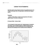
Figure 16 is the computed function of the ACF and the PACF from the Ex-Post data. It shows that from the ACF the lags gradually decays and that from the PACF, after the first lag cuts off to zero therefore showing that the data is non-stationary. As a result the data is differenced by one to make the data stationary.

Further Identification and Estimating the Parameters

Once an appropriate model has been selected, the parameters of each model must be estimated. This stage provides some warning signals about the adequacy of the model, if the estimates do not satisfy certain conditions, that model should be rejected. The parameters of the ARIMA model are estimated by minimising the sum of squares of the fitting errors.

Table 15: ARIMA Estimation

Diagnostic Checking

At this stage, each model is checked before it is forecasted to find the best model. An adequate model is one where the residuals cannot be used to improve the forecast. “That is, the residuals should be random.”

The model that has all criteria needed is a good

1. Is parsimonious
2. Is stationary
3. Is invertible
4. Fits the data sufficiently at the estimation period (lowest MSE)
5. High quality estimated coefficients
6. Statistically independent residuals

---

Table 16: ARIMA Strengths and Weaknesses

Table 16 is the Strengths and Weakness Table from the estimated models calculated from Table 15. From each of the estimated model the strengths and weaknesses were noted in order to find the best model to forecast the data. When estimating the models, two models stood out; ARIMA (2 1 0) and ARIMA (1 1 2). ARIMA (1 1 2) would have been the best model to use to forecast the data, however, despite having the lowest Mean Squared Error it did not have a p-value of at least 10% therefore was not sufficient enough to use. As a result, the next best-estimated model was ARIMA (2 1 0) because it had a low Mean Squared Error and a p-value of at least 10%, therefore making it an ideal estimate to forecast the data. Figure 17 shows the forecast of ARIMA (2 1 0).

Figure 17: ARIMA (2 1 0) Forecast

Figure 17 shows the graph of the optimal estimated ARIMA model for both one-step and four-step. Both one-step and four-step follow a very similar pattern to the Ex-Post, however, the four-step shown by the green dashed line reacts to the realisation at a later point of the data. The one-step ARIMA shows a more accurate forecast of the Ex-Post because during some points of the data there are points where the ARIMA is on the Ex-Post data.

Table 17: ARIMA Mean Squared Error

In order to see how accurate the ARIMA model is the MSE has been calculated for both the one-step and four-step model. The one-step model shows a better forecast than the four step, however, the four step model too shows a good forecast of the model compared to the previous four-step models.

Figure 18: One-Step - Naive Trend Vs ARIMA

Figure 18 shows the comparison between the benchmark Naive Trend Model and the ARIMA model for the one-step short-term forecast. The green dashed line represents the ARIMA model and the red line for the Naive Trend. The ARIMA model has some data points that are smoother and closer to the Ex-Post than the Naive Trend, however, the Naive Trend still follows a close pattern to the realisation. To see how close the patterns on the two models are, Figure 19 shows a zoom in of the two models.

Figure 19: Zoom In - Naive Trend Vs ARIMA

Figure 19 shows the Zoom In on the Naive Trend and the ARIMA model for the one-step. On average, the ARIMA model performs better than the Naive Trend, as it is closer to the Ex-Post. This is supported by Table 19, which shows the calculated MSE of both the models.

Table 18: MSE One-Step - Naive Trend Vs ARIMA

The table shows that the ARIMA model is a much more accurate forecast than the Naive Trend model.

Figure 20: Four-Step - Naive Trend Vs ARIMA

Figure 20 is the comparison of the four-step Naive Trend against the ARIMA. It is evident from the graph that the ARIMA model denoted by the green line is a much smoother fit than the Naive Trend. The model follows a much closer pattern to the Ex-Post data and there is less variation and volatility compared to the Naive Trend.

Table 19: Four-Step MSE - Naive Trend Vs ARIMA

Table 20 is the results of the calculated MSE for the Naive Trend and the ARIMA four-step model. The ARIMA performs significantly better than the Naive Trend and is supported by the forecast of Figure 20.

Figure 21: Four-Step - Brown Vs ARIMA

Even though the Naive Trend was used as the benchmark model, the Brown’s four-step model performed better than the Naive Trend and the Holt’s method. Therefore, Figure 21 is a comparison of the Brown against the ARIMA and despite the Brown’s model performing better before the ARIMA model is still the more accurate forecast. Table 21 shows that the four-step ARIMA performs six times better than the Brown’s model and therefore making the ARIMA the best long-term forecast.

Table 20: MSE Four-Step - Brown Vs ARIMA

---

Error Results

Table 21: One-Step Errors

Table 21 is a of all the error terms for the one-step short-term model. The mean squared error has been used throughout the report to calculate the accuracy of the models. The ARIMA model was be more accurate model for the one-step forecast and if we look at the other error measures paying more attention to the Theil-U statistic, it confirms that the ARIMA model is the best forecast for the short-term. The Naive Trend model has been used, as the benchmark model therefore is equal to one. Both the Brown and Holt’s model are more accurate than the Naive Trend and therefore supporting the mean squared error because of the smoothing constants and therefore making the forecast more accurate. However, the ARIMA is smaller and therefore showing that the model is a more accurate forecast because there are more variables that are taken into consideration, therefore making it the better model.

Table 22: Four-Step Errors

Table 22 is the four-step long-term error results from the estimated models. The ARIMA model again produced the more accurate forecast measured by the mean squared error. The long-term forecast for the Brown and Holt’s model was better forecast than the Naive Trend but the difference was not as great as the ARIMA. The ARIMA model was significantly better than all the other forecasted models therefore making it the best forecast. By looking at the Theil-U statistic, the Naive Trend is used as the benchmark model and both Brown and Holt’s model are a slightly better forecast. The ARIMA once again is a significantly accurate forecast than all the other models.

Looking at the Mean Absolute Deviation, the Mean Absolute Percentage Error and the Mean Percentage Error, all the Error terms supports the Mean Squared Error and the Theil-U statistics, for the Naïve Trend model being the least accurate model and the ARIMA being the most accurate. The figures for the mean percentage error are in percentage terms, therefore hide the magnitude of the actual errors, and as a result show very low figures.

---

Conclusion

Several different models have been used to forecast the future time series. This report has examined; the Decomposed time series, the Naive Trend and the Naive Rate of Change, Brown Double Exponential Smoothing Method, Holt’s two-parameter method and a non-seasonal ARIMA model. Canada’s quarterly GDP data were of constant prices from 1980 quarter 1 to 2007 quarter 1, which was divided into two periods; an estimation period and a test period. The estimation period was used to choose the parameters of the models that would be used for Ex-Post forecasting. The worst model that was used to forecast the test period was the decomposed time series. This was because the trend data forecasted a straight line and does not follow a close pattern to the test period. In addition, the decomposed time series does not adjust to any change in the data and when calculating the mean squared error it was the highest figure and the least accurate forecast of the in sample forecasts. The most accurate model was the ARIMA (0 1 2) model for both the one-step short-term forecast and the four-step long-term forecast because it gave us the lowest mean squared error. The Theil-U statistic was also used as a Error forecast as an extra measure of accuracy, which had supported the results of the mean squared errors. Throughout the report, the Mean Squared Error was used as a measure of accuracy and from each of the models the parameters were altered until the lowest possible mean squared error was attainable. For the Brown and Holt’s model the smoothing constant of alpha, and beta (Holt’s model only) were altered until the lowest MSE was found and then from the result the model was forecasted. Both the exponential smoothing methods are a very good forecast of the data because extra variables are added to make a accurate forecast. Therefore, the models should not be disregarded when it comes to forecasting. Even though the Naïve Trend model is the least accurate forecast next to the decomposed time series, it is a very quick and simple method of forecasting a time series.. Therefore to conclude the report, the best model to use to forecast Canada’s quarterly GDP data is the ARIMA (0 1 2) model for both the short and long-term forecast.

Bibliography

Hanke, J. E., & Wichern, D. W. (2008). Business Forecasting, 9th Edition. Pearson Prentice Hall International Edition.

Meyer Ruth and David Krueger, (2006), A Minitab Guide to Statistics, Third edition, Prentice Hall.

Niemira M P & Philip A Klein, (1994), Forecasting Financial and Economic Cycle, John Wiley & Sons, Inc.

OECD. (2010, December). GDP, Total and Expenditure Components. Retrieved January 2011, from Organisation for Economic Co-operation and Development (OECD): http://stats.oecd.org/Index.aspx?querytype=view&queryname=206

Pindyck R S & Daniel L.Rubinfeld, (1998), Econometric Models and Economic Forecasting, Fourth Edition, McGraw-Hill, Inc.

Richard A. Brealey, S. C. (2008). Principles of Corporate Finance, 9th Edition. McGraw-Hill.

Zhang, W. (2010). Business Financial Forecasting - With a Minitab Guide. Manchester: MMU.

---

Appendix

Appendix 1: One-Step Data

---

Appendix 2: Four-Step Data

---