indifference curve analysis

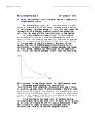
The marginal rate of substitution (MRS) = change in good x / change in good y.

Again using the first diagram, the marginal rate of substitution between good x and good y is-

MRS= -3/3 = 1

The rule is to ignore the sign. The reason why the marginal rate of substitution diminishes is due to the principles of diminishing marginal utility, where this principle states that the more units of a good are consumed, and then additional units will provide less additional satisfaction than the previous units will. Therefore as relating it back to the example above as a person consume more of one good ( i-e, work) then they will receive diminishing utility for that extra unit (satisfaction). Hence, they will be willing to give up less for their leisure to obtain one more unit of work. The relationship between marginal utility and the marginal rate of substitution is often summarised with the following equation;

MRS = Mux/Muy

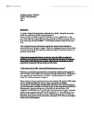
It is possible to draw more than one indifference curve on the same diagram. If this occurs then, it is known as an indifference curve map. If income is held constant, and the price of one of the goods changes then the slope of the curve will change. In other words, the curve will pivot. This is shown in the figure below:

The general rule is that indifference curves further to the right line D & E show combinations of the two goods that yield a higher utility, while the curves to the left A & B shows the combination that has been consumed low level of utility.

The budget line is in important component when analysing concumer behaviour. The budget line illustrates all the possible combinations of two goods that can be purchased at given pricess and for a given consumer budget. Remember, that the amount of a good that a person can buy will depend upon their income and the prices of the good. This outlines the contraction of a budget line and how to change in the determinants will affect the budget line.

For example, lets assume we have a budget of £60, and £2 per unit of X and £1 per unit of y. With a limited budget the consumer can only consume a limited combination of x and y.

If consumer income increases then the consumer will be able to purchase higher combinations of goods. Hence, an increase in income will result in a shift in the budget line. This is illustrated in the figure below. Note that the price remains the same for both of the goods; therefore, the increase will result in the parallel shift in the budget line. For example, let us assume consumer increased to £90.

If for instance the consumer income fell then there would be a corresponding parallel shift to the left to represent a fall in the potential combinations of the two goods that can be purchased.

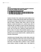
If income is held constant, and the price of one of the goods changes then the slope of the curve will change. In other words, the curve will pivot. This is shown in the diagram below:-

The reduction of the price of good x from £2 to £1 means that on a fixed budget of £60, the consumer could purchase a maximum of 60 units, as opposed to30. Note that the price for the good y remains same and fixed. Hence, the maximum point for good y will remain fixed. The indifference curve analysis combines two concepts, which are indifference curve and budget line.

The first stage is to compose the indifference curves and budget line to identify the consumption point between two goods that a rational consumer with a given budget would purchase.

A rational, maximising consumer would prefer to be on the highest possible indifference curve given their budget constraint. This point occurs where the indifference curve touches the budget line. In the case of the above diagram this would be the optimum consumption point occurs at point E on indifference curve B. Indifference analysis can be used to analyse how a consumer would change the combination of two goods for a given change in their income or the price of the good.

The next section looks at the income and substitution effect of a change in price. If we assume that the good is normal, then the increase in price will result in the fall in the quantity demanded. This is for two reasons; the income effect, which have a limited budget, therefore can purchase lower quantities of the good and secondly the substitution affect which swaps with alternative goods that are cheaper. These two processes can be visualised using indifference analysis as shown in the diagram below.

Due to the price of good x increasing, the budget line has pivoted from B1 to B2 and the consumption point has moved. The decrease in the quantity demanded can be divided into two effects; the substitution effect is when the consumer switches consumption patterns due to the price change alone but remains on the same indifference curve. To identify the substitution effect, a new budget line needs to be constructed. The budget line B3 is added, this budget line needs to be parrelel with budget line B2 and tangential to C1. There the movement from Q1 to Q2 is purely due to the substitution effect. The second effect which is the income effect highlights how consumption will change due to the consumer having a change in purchasing pwer as a result of the price change. The higher price means the budget line is B2,hence the optimum consumption point is Q2. This point is on a lower indifference curve C2. Therefore, in the case of a normal good, the income and substitution effect work to reinforce each other.

If for instance the consumer income fell then there would be a corresponding parrelel shift to the left to represent a fall in potential combinations of the two goods that can be purchased.

---