RDIPH was included as economic theory suggests that with increased income comes increased demand. Therefore, if beef is a normal good I would expect there to be a positive coefficient. However, there is the possibility that beef may be an inferior good and so could have a negative coefficient. As people have more money, they would spend it on more luxurious goods than beef.
TIME was included to show the effects of changes in consumer preferences during the period- 1967-95. I would expect this to have a negative coefficient due to three factors:
1) Vegetarianism, causing a general shift away from meat.
2) The development of a healthier eating culture with people opting for healthier options rather than beef.
3) The effects of BSE with the fallback of this being and public loss of confidence in beef altogether.
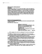
My initial model was:-
QB= a + b RPB + c RPP + d RPC + e RDIPH + f TIME + e
a is the intercept. This isn’t shown in my results as it is not needed. e is the random variable
Number in bold=t ratio
Number in brackets=standard error
Other number=coefficient
Evaluation of models.
T test. Testing significance- Model 1
RPB Ho:b=0- fluctuations have no effect. This is not what is expected
H1:b<0- if the price goes up quantity goes down. Downward sloping graph from left to right this is to be expected.
t= (B-B )/SE (B )
t= (-0.419-0)/0.141=-2.972- I will now just use the table from now on
Degrees of freedom= N-K N= number of years
K=variables
=29-5
=24
t value of -2.972 with 24d of f is statistically significant on a 1tt (as coefficient as expected) at a level of 0.005. Therefore I can reject the null hypothesis with a 5 in 1000 chance of being wrong. This strongly suggests that the results are as expected and would make a graph sloping downwards from left to right in line with economic theory.
RPP Ho: c= 0
H1: c> 0
2tt as the results weren’t as expected, the coefficient says that if RPP is increased then consumption for beef would go down, this isn’t in line with economic theory. This may not be a significant result. The t test will say.
t= -0.779 with 24d of f is not significant. We cannot reject the null hypothesis. Not significantly different from 0. fluctuations in RPP do not significantly affect the consumption of beef.
RPC Ho: d=0
H1: d>0
Again a 2tt as the coefficient isn’t as expected, -0.116 with 24 d of f. 0.116 is not significantly different from 0. fluctuations in RPC will not significantly affect the consumption of beef.
RHDIP Ho: e=0
H1: e>0
2tt as coefficient isn’t as expected. t ratio -1.466 with 24 d of f is only significant at the 10% level. This is not a very significant result as there is a 10% chance of being wrong if I reject the null hypothesis. This is not a significant result however, as I am only taking significance at a 5% level to being significant.
If income goes up then the consumption of beef goes down. This suggests that beef is an inferior good with people preferring to spend their money on other goods if they can afford to.
TIME Ho: f=0-says there is no trend
H1: f>0-says that there could be a positive or negative relationship.
-0.659 with 24 d of f is not significant therefore we can’t reject Ho.
R² says that the model explains89% of the demand for beef. This isn’t a very good model.
Model 1 gave some surprising results. Neither of the substitutes caused a significant change in the demand for beef, suggesting that they have completely independent demand functions. Maybe this was due to the fact that pork and chicken are white meats, and they are not considered as substitutes for beef. RHDIP says that there is a no significant trend or relationship to buy beef as income increases, this is surprising as I consider beef to be a superior meat, it does, however, make me wonder about the effects of BSE on consumption. TIME not being significant surprises me as I would have expected to see a trend away from beef in lieu of BSE.
Model 2 is;
QB= a +bRPB+cRPL+dRPP+eRPC+fTIME+e
In model 2 I included the other dark meat available lamb- RPL. I would expect to find a positive relationship between them, as lamb consumption goes up beef consumption goes down and vice versa.
t tests:
RPB Ho: b=0
H1: b>0 1tt 2.266 is significant reject Ho. Not as significant.
RPL Ho: b=0
H1: b>0 2tt -0.188 not significant.
RPP-not significant
RPC-not significant
TIME-not significant
This was interesting as it shows that the consumption of lamb is not responsive to the consumption of beef.
For model 2 the t ratios on the whole were of greater significance than mode 1,however, there were better results for R² in model 1.
Model 3 was an attempt to take into account last year’s consumption with the lagged time variable QB1.
QB= a + bRPB+ cQB1
He results for this test were not significant which tends to dispel the theory that a positive coefficient would be found with consumption to be high this year if it was last year.
Model4 is QB=a+bRPB
This also created an insignificant relationship.
In hindsight, perhaps I have chosen the wrong models to work with as it seems that a model that looked like this would have been better
QB= a+bRPB+cRPP+dRPC+eRDIPH+fTIME+gQB1e
This would have been the best to do as it would not only have showed the relationship between all the substitutes, the effects of consumer change over the years and real disposable income but also last years consumption.
Having not done this, however, I will be using model 1 for my forecasting.
Elasticties
Elasticities show how responsive a product is to changes in price. There are different types of elasticities and I intend to try and work out three elasticities- price, cross and income. The price elasticity is how responsive a product is to changes in price, in our case beef. Cross elasticity is how responsive a product is to the change in other goods. Income elasticity is how responsive a product is to a change in income.
Price elasticity of demand- % change in Q P
% change in P x Q
= 1 P
0.419 x Q
this is Elastic as demand changes with price if price goes down then demand increases.
Cross elasticity of demand- % change in Q P
% change in price of alternate good x Q
RPP= 1/0.218 x RPP/Q
RPC= 1/0.333 x RPC/Q
Although one would presume that a change in price of a substitute good would effect the demand for beef, it is not the case here. Oddly enough there seems to be very little in terms of a relationship between the two- in elastic.
Income elasticity of demand- % change in Q income
% change in Income x Q
= 1/0.021 x income/Q
Again this proves to be inelastic, as there doesn’t seem to be a relationship whereby if income goes up then consumption will not go down.
Therefore after consulting the t ratios the reliability of these estimates are good.
Forecasting
There is a graphical forecast on the sheet labeled overleaf. This forecast is not very accurate, where the actual curve starts to dip the forecast starts to rise, and when the actual curve starts to rise, the forecast starts to dip. This could be for a number of reasons; firstly I would wonder about the effects of BSE and the fact that in 1997 in the actual curve there is a massive dip in consumption, funnily enough when BSE was at its peak. The fluctuations in the curve, however could have been because of limitations in the model- for example it doesn’t include complementary goods such as Yorkshire puddings or beef stock or vegetables, if there is a fall in their price an increase in beef consumption would be expected. The average error for my forecasting over the five post estimation years is 14.823.
Possible improvements
Possible improvements include, including lamb on my primary model, and having a subperiod of before during and after the BSE crisis, this would have showed me how much the crisis affected the general results. And lastly, if the file had contained more variables such as complementry goods, this would help in reaching a more complete model.
Flegg T(2001) lecture notes
Jacues A (1999) Mathmatics for Economics and Business, Harlow, Pearson Education Limited
Sloman J (2000)Economics, Harlow, Pearson Education Limited