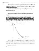
Lipsey's assumption was that dW/W=f [(DL-SL)/SL]. The graph of this function is represented in Figure 3. The speed of adjustment or the rate of change on wages dW/W is on the vertical axis and the excess demand for labour relative to the supply of labour [(DL-SL)/SL] on the horizontal axis. The further away we go from the origin the larger the excess demand for labour and the higher the speed of change of money wages.
As it was assumed that there is a strong inverse relationship between vacancies and unemployment, it will be enough to monitor just unemployment as it is a proxy for excess demand for labour. In Figure 4, the inverse relationship between recorded unemployment and excess demand for labour can be observed. Point B coincides with the equilibrium wage level W0 from Figure 1, where the excess demand is zero as well.
The final diagram in Figure 5 represents the derived Phillips curve created by combining the assumptions made in Figures 3 and 4. It depicts the relationship between the unemployment and the wage change rates.
Lipsey's theory of the Phillips curve was further developed by P. Samuelson and R. Solow. They generalised this concept by replacing rate of change of wages with inflation represented by dP/P in Figure 6.
The Phillips curve was recommended to economic policy makers as an instrument that would allow them to formulate policy programs with alternative combinations of unemployment and inflation rates. As Samuelson and Solow (1960) expressed it, policy makers would face a 'menu of choice between different degrees of unemployment and price stability.' "(Frisch 1983, p.41)
Governments want to maximise social welfare by achieving low rates of inflation and unemployment, this is done by inserting indifference curves which represents government preferences. The indifference curves show different combinations of inflation and unemployment that yield the same level of social welfare, and the closer the indifference curve to the origin the higher the social welfare. At the indifference curve I0 the social welfare is maximised because we can't increase welfare any further (to I3 for example) given this Phillips curve.
I1 and I2 show different preferences of policy makers. I1 shows a government which is adverse to high unemployment and prefers low unemployment to low inflation. By contrast, I2 shows a government which is adverse to high inflation and prefers to have low inflation rather than low unemployment. This kind of policy tends to be preferred by Germans because they experienced hyperinflation in the inter-war period when the Deutsche Mark was highly devalued.
In the 1960's policy makers considered the Phillips curve model useful for predicting the behaviour of the economy. However E. Phelps (1967) and M. Friedman (1968) strongly criticised this model.
"Their challenge was to ask: how could the rate of change of nominal variables, such as nominal wages and prices, be related to real variables such as employment, unemployment, and output in the long run?" (Burda 2005, p.286). They criticised Lipsey's theory because it doesn't take account of inflationary expectations.
At the time, policy makers didn't listen to Friedman's and Phelps' arguments. The next decade brought economic instability when both the inflation and unemployment rates were rising at the same time, which was referred to as stagflation. The Phillips curve was consistently failing to explain these events; it suffered an 'empirical breakdown'.
Policy makers were looking for a new model which would provide an explanation for the recent economic downturn. A plausible one was proposed by Friedman and Phelps, the expectations-augmented Phillips curve. In 1979 after the stagflation period, Margaret Thatcher became prime minister and as soon as she was elected, she arranged a meeting with Milton Friedman implying the inclination to adopt his vision of a stabilising policy.
Friedman argues that Lipsey's Phillips curve works only in the short-run, where economic agents' expectations lag behind the actual rate of inflation. Figure 7 shows this case. At the initial point A, inflation and unemployment rates are P1, U1 respectively. The government attempts to achieve a lower unemployment level by increasing the money supply, this pushes up inflation from P1 to P2 and lowers unemployment from U1 to U2, bringing us to point B. However, the decrease in unemployment will only be temporary because the expectations about inflation lag behind the actual inflation rate, meaning that workers who got jobs (U1 to U2) perceived the increase to be in their real wages. In fact all the other nominal variables increased as well, leaving the real magnitudes unchanged. This logic would work if people suffered from "money illusion". In real life people's expectations catch up and they realise that their real wage remained constant, and the level of unemployment will fall back to its initial U1 level, making point C the new equilibrium. This equilibrium rate of unemployment U1 is in fact the natural rate of unemployment UN, which is "the long-term sustainable rate of unemployment within an economy." (Pearson Education, 2005). The natural rate of unemployment includes frictional unemployment, which represents people who are in the process of switching jobs, structural unemployment is caused by the unsuitability of workers' skills to the available jobs and voluntary unemployment.
In the long run the equilibrium level of unemployment will always be equal to the natural rate of unemployment, making the long run Phillips curve a vertical line, which is shown in Figure 7 as an increase in money supply eventually leads to point C because expectations always catch up. This process will constantly occur when the money supply is increased hence the long run Phillips curve being a vertical line. One policy implication of this finding is that lower unemployment is only temporary but at the cost of permanently higher rate of inflation.
The Post Keynesians developed on this idea formulating their "distribution view". They agreed with Friedman's aphorism that inflation is always a monetary phenomenon. They argued that inflation can only occur in economies that use money to organise the production and exchange processes. "Inflation is a symptom of a fight over the distribution of current income." (Davidson 1994, p.149) In the case of firms, they change the distribution of income in their favour by increasing the prices, workers react by demanding higher wages; this spiral causes inflation.
In the natural rate of unemployment hypothesis offered by M. Friedman, rate of inflation is formulated as:
πt=f(ut)+πt*
where the actual rate of inflation is πt, πt* is the expected inflation and f(ut) is a function of the excess demand in the goods and labour markets.
The expected rate of inflation is generated by adaptive expectations:
πt*=kπt-1+(1-k)πt-1*
where the expected rate of inflation for period t is the weighted average (k is the weight) between the actual rate of inflation in the preceding period πt-1 and the expected rate of inflation in preceding period πt-1*. In this case the expectations of the rate of inflation are entirely based on past data.
Lucas and others questioned the rationality of the adaptive expectation hypothesis. To suppose people behave in the way where their expectations are always lagging behind isn't plausible. This suggests economic agents are always under-predicting expectations. A more sensible strategy would be to take into account other relevant information like macroeconomic indicators: interest rates, government policy etc. The concept behind rational expectations is that adaptations to new inflation rates happen immediately, thus making the short run Phillips curve the same as the long run.
The concept of the Phillips curve evolved significantly since its conception. The initial theory proved to be valid just in the short run, but due to changing expectaions it tranformed into the vertical long run curve. This shows how the view on economic agents' behaviour evolved.
Bibliography
BURDA, Michael C., WIPLOSZ, Charles, 2005. Macroeconomics a European text. 4th ed. New York: Oxford University Press.
CHAMBERLIN, Graeme and YUEH, Linda, 2006. Macroeconomics. London: Thomson.
COBHAM, David, 1998. Macroeconomic analysis: and intermediate text. 2nd ed. London: Longman.
DAVIDSON, Paul, 1994. Post Keynesian Macroeconomic Theory. Aldershot (England): Edward Elgar Publishing.
FRISCH, Helmut, 1983. Theories of inflation. Cambridge: Cambridge University Press.
PEARSON EDUCATION, 2005. Glossary. Available at: http://wps.pearsoned.co.uk/wps/ media/objects/2499/2559960/glossary/glossary.html [Accessed 07 March 2010].
SHAW, G.K., MCCROSTIE, Michael and GREENAWAY, David, 1997. Macroeconomics: theory and policy in the UK. 3rd ed.Oxford: Blackwell.
2010 | ECON20011 | Macroeconomics | level 2 | page