The increase in income leads to the shift of the curve from AB to CD on the diagram, a parallel movement. The effect will be that to open up the consumer the possibility of buying bundle of goods yielding more utility than was obtained before. The equilibrium will shift from E to F, a shift right. This shows that income has expanded e.g. the income expansion plan (IEP) which would be E to F. The indifference curve shifts from IC to IC2. So now the maximum of fish has gone up by 2 to 22 fish and beans have gone up by 3 to 36 as income has increased to £110. These are maximums and so more can be purchased.
The price of fish goes up by 25%?
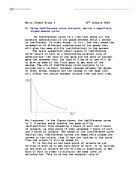
We have to calculate the fish price first, so£5 X 25/100 = £1.25 then you add this to the original price so it equals £6.25. Then we have to calculate to plot the graph so £100/£6.25 = 16 fish and beans stay the same at 33. All this can be seen in Figure 3.
The indifference curve shifts from IC to IC2 shifts to the left. This is because purchasing power has diminished. As the person prefers fish more, will be more affected by the price increase this can be shown in the diagram might even shift from buying fish now purchasing more beans than fish. The equilibrium has just moved down from 10 to 8 for fish (E to F).
There is an aggressive advertising campaign?
The aggressive advertising campaign will mean that more people will be buying the two goods. Which will mean the indifference curve will shift to the right. If the advertising is more to buy beans then more people will buy beans with there income and if the advertising is to buy more fish then people will buy fish more. So if they have a income of £100 and fish is £5 and beans are £3, then if aggressive advertising then they will buy equal amounts of both or just spend all of there income on one product fish or beans.
What are weaknesses of the Hicks-Allen indifference curve analysis?
Indifference curves are showing alternative combinations of two products, each of which gives the same utility or satisfaction. (e.g. fish and beans).
One of Hicks' most contributions is the demand theory he developed using indifference curves. The advantage of his demand theory is the realistic nature of its assumptions. Consumers must state whether they prefer one option to another, or whether they are indifferent between any two options they are asked to choose. In other words, consumers simply rank their options in order of preference, rather than having to specify how much utility one option provides compared with another. If your actually creating a indifference curve it is virtually impossible, since it would involve a consumer trying to think of different combinations of goods and trying to decide which gives great satisfaction, it just wouldn’t work.
An illustration will show how indifference curves work. E.G. Suppose a consumer, Alice, is asked to choose between two bundles, each containing different amounts of milkshakes and hamburgers consumed during a week. For example, Alice may choose between bundles a 4 milkshakes along with 3 hamburgers and bundle b 3 milkshakes along with 4 hamburgers. Given her preferences, she may select either a or b, or she may decide she is indifferent between a and b, because each bundle gives her the same level of utility.
In any application of neoclassical theory of consumption, one of the key problems is that indifference curves which provide it’s theoretical core, cannot be observed we cannot, as it were, peep into the heads of each consumer and find out their preferences among the vast array of consumption goods that are on offer. We cannot plot an individual’s indifference curve using real world data.
Although the advantages of the indifference-curves approach are important, the theory has indeed its own severe limitations. The main weaknesses of this theory are its axiomatic assumption of the existence and the convexity of the indifference curves. The theory does not establish either the existence or the shape of the indifference curves. It assumes that they exist and have the required shape of convexity. Furthermore, it is questionable whether the consumer is able to order his preferences as precisely and rationally as the theory implies. Also the preferences of the consumers change continuously under the influence of various factors, so that any ordering of these preferences, even if possible, should be considered as valid for the very short run.
Another defect of the indifference curves approach is that it does not analyse the effects of advertising, of past behaviour (habit persistence), of stocks, of the interdependence of the preferences of the consumers, which lead to behaviour that would be considered as irrational, and hence is ruled out by the theory. Furthermore speculative demand and random behaviour are ruled out. Yet these factors are very important for the pricing and output decisions of the firm.
More limitations are consumers may not behave rationally and may not give careful consideration to the satisfaction they can get from consuming the goods. And certain goods are only purchased every now and again and then only one at a time e.g. cars and televisions. Indifference curves are based on the assumption that marginal increases in one good can be traded off against marginal decreases in another. This will not be the case with consumer durables.
BIBLIOGRAPHY
Robert S.Pindyck, Daniel L.Rubinfeld (2001), Microeconomics Fifth Edition, United States of America.
David Begg (1997), Economics Fifth Edition, McGraw Hill, UK.
A Griffiths and S Wall, Intermediate Microeconomics: Theory and Applications, Longman, 2nd ed, 2000.
JM Perloff, Microeconomics, Addison Wesley, 2nd ed, 2000.
HRVarian, Intermediate Microeconomics, 4th ed, W.W. Norton, 1996.
J.Hicks, Value and Capital (Oxford University Press 1946) 2nd ed.
E.J. Mishan, Theories of Consumers Behaviour: A Cynical View. Economica (1961).
Lectures 1 and 2.