P(£)
a
5 b
4
D
10 20 Q
This is illustrated in the above figure. Demand is elastic between points a and b. a rise in price from £4 to £5 causes a proportionately larger fall in quantity demanded: from 20 million to 10 million. Total expenditure falls from £80 million (the striped area) to £50 million (the pink area). (J. Sloman, economics, pg. 53)
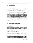
On the other hand, if the percentage change in the quantity demanded is less than the percentage change in price, then the value of elasticity of demand is less than one and therefore we have inelastic demand. In this case, the change in price has a bigger effect on the total consumer expenditure than does the change in quantity. In other words, total consumer expenditure changes in the same direction as price. This is illustrated in the following figure. Demand is inelastic between points a and b. A rise in price from £4 to £8 causes a proportionately smaller fall in quantity demanded: from 20 million to 15 million. Total expenditure rises from £80 million (the striped area) to £120 million (the pink area). (J. Sloman, economics, pg. 53)
P
8
4
D
15 20 Q
Another concept of elasticity of demand is when (PED) =0. At this point, we have totally inelastic demand, which is shown by a vertical line as it is illustrated in the following figure.
P D
P2 b
P1 a
0 Q1 Q
In totally inelastic demand, regardless of what happens in price, quantity demanded remains the same. It is obvious though, that the more the price rises, the bigger will be the level of total expenditure. There are many goods, which have a totally inelastic demand at all prices. These are goods that people really need and no matter how big their price is they are in a way forced to buy them. Such a good that has a low elasticity of demand is insulin. Insulin is of such importance to some diabetics that they will buy the quantity that keeps them healthy at almost any price. Even at low prices, they have no reason to buy larger quantity.
On the contrary, we have the indefinitely elastic demand, when (PED) = ∞. Diagrammatically, this is shown by a horizontal straight line. At any price above P1 in the following figure, demand is zero. On the other hand, at P1, or any other price below, demand is ‘indefinitely’ large.
P
a b
P1 D
0 Q1 Q2
Unlikely though the above demand curve may seem, it is common for an individual producer. An example of a good that has high elasticity of demand, almost indefinite, is ballpoint pens from the university bookshop or from the newsagent’s shop close by. If the two shops offer pens for the same price, some people buy from the one and some from the other. Nevertheless, if the bookshop increases the price of pens, even by a small amount, while the shop close by maintains the lower price, the quantity demanded from the bookshop will fall to zero.
There is also the unit elastic demand, when (PED) = 1. This is where price and quantity change in exactly the same proportion. Any rise in price will be exactly offset by a fall in quantity, leaving total consumer expenditure unchanged. In the following figure, the striped area is exactly equal to the pink area: in both cases, total expenditure is £800. Such a curve is called a rectangular hyperbola. The reason for its shape is that the proportionate rise in quantity must equal the proportionate fall in price and vice versa. As we move down the demand curve, in order for the proportionate change in both price and quantity to remain constant, there must be a bigger and bigger absolute rise in quantity and a smaller and smaller absolute fall in price. For example, a rise in quantity from 200 to 400 is the same proportionate change as a rise from 100 to 200, but its absolute size is double. A fall in price from £5 to £2.50 is the same percentage as a fall from £10 to £5, but its absolute size is only half.
P
20
8 D
40 10 Q
Substitute is a good that can be used in place of another good. The closer the substitute for a good or service, the more elastic is the demand for it. For instance, housing has few real substitutes such as sleeping on a friend’s floor, in a hostel or on the street. As a result, the demand for housing is inelastic. On the contrary, metals have good substitutes such as plastics and car travel has substitutes in public transport, so the demand for these goods is elastic. In everyday language, we call some goods, such as food and housing, necessities and other goods, such as exotic vacations, luxuries. Necessities are goods that have poor substitutes and that are crucial for our well - being, so generally they have inelastic demands. Complement is a good used in conjunction with another good. Some examples of complements are hamburgers and chips, party snacks and drinks, cars and petrol, PCs and software.
The quantity of any good that consumers plan to buy depends on the prices of its substitutes and complements. We measure these influences by using the concept of the cross elasticity of demand. The cross elasticity of demand is a measure of the responsiveness of the demand for a good to a change in the price of a substitute or complement, other things remaining the same. It is calculated by using the formula:
Cross elasticity percentage change in quantity demand
of demand percentage change in the price of a substitute or a complement
The cross elasticity of demand is positive for a substitute and negative for a complement. The following figure makes it clear why.
Price
of oil
D1
D0
D2
0 Quantity of oil
When the price of coal, a substitute for oil, rises, the demand for oil increases and the demand curve for oil shifts rightward from D0 to D1. Because an increase in the price of coal brings an increase in the demand for oil, the cross elasticity of demand for oil with respect to the price of coal is positive. When the price of a car, a complement for oil, rises, the demand for oil decreases and the demand curve for oil shifts leftward from D0 to D2. Because an increase in the price of a car brings a decrease in the demand for oil, the cross elasticity of demand for oil with respect to the price of a car is negative. Therefore, positive values identify substitutes and negative values identify complements. (Michael Parkin, Melanie Powell, Kent Matthews, economics, pg. 106).
Finally, the demand of a particular good may also change because of the income. This is another concept of elasticity of demand, the income elasticity of demand, which is a measure of the responsiveness of demand to a change in income, other things remaining the same. It is calculated by using this formula:
Income elasticity percentage change in quantity demanded
of demand percentage change in income
Income elasticities of demand can be either positive or negative and fall into three interesting ranges:
- Greater than one. As income increases, the quantity demanded increases, but the quantity demanded increases faster than income. Some examples of income elastic goods are extreme luxuries such as ocean cruises, international travel, jewellery and works of art. Nevertheless, many other non-necessity goods are income elastic, such as the services of hairdressers and accountants. The following figure illustrates the income elasticity greater than one.
Quantity
demanded
0 Income
Quantity
Demanded
0 Income
The above figure shows an income elasticity of demand that is between zero and one. In this case, the quantity demanded increases as income increases, but income increases faster than the quantity demanded. Examples of goods in this category are food, clothing, furniture, newspapers and magazines.
- Less than zero. In this case, the quantity demanded increases as income increases until it reaches a maximum at income m. Beyond that point, as income continues to increase, the quantity demanded declines. The elasticity of demand is positive but less than one up to income m. Beyond income m, the income elasticity of demand is negative. Examples of goods in this category are small motorcycles, potatoes, rice and bread. Low-income consumers buy most of these goods. At low-income levels, the demand for such goods increases. But as income increases above point m, consumers replace these goods with superior alternatives. For instance, a small car replaces the motorcycle; fruits, vegetables and meat begin to appear in a diet that was heavy in bread, rice or potatoes. The following figure shows an income elasticity of demand that eventually becomes negative.
Quantity
demanded
0 m Income
Drawing a conclusion, elasticity of demand has many different concepts, which help both producers and consumers in economic decision-making.