The "surprise" aggregate supply curve - Assess Lucas' theory on monetary misperceptions.

University Degree Business and Administrative studies

The “surprise” aggregate supply curve

Assess Lucas’ theory on monetary misperceptions

Throughout our studies in macroeconomics we have come across various different models that are intended to describe the connection, in terms of cyclical fluctuations, between nominal and real variables. Understanding this connection is extremely important, as it governs the effect of monetary policy on employment, output and other crucial real variables. In this essay we will look at the theory of monetary misperceptions developed by Robert.E.Lucas. His theory builds upon the fact that individual sellers do not have complete information concerning the state of the economy and so form expectations rationally. There are many competing theories, each of which has attracted significant attention. No theory has yet been developed which precisely explains the period by period dynamics of aggregate supply. First, lets take a look at the origins of the models we will later discuss.

In 1936 John Maynard Keynes began the Keynesian revolution with his book The General Theory of Employment, Interest and Money. Keynes proposed a new way to analyse the economy, which he presented as an alternative to classical theory. His vision of how the economy works quickly became a center of controversy. Yet as economists debated The General Theory, a new understanding of economic fluctuations gradually developed. In The general Theory, Keynes proposed that an economy’s total income be, in the short run, determined largely by the desire to spend by households, firms and the government. The problem during recessions and depressions, according to Keynes was inadequate spending. The Keynesian cross is an attempt to model this insight.

In 1937 John Hicks introduced the IS-LM model which generally represents Keynes’s General Theory in the form of a system of simultaneous equations. A problem was that it was unable to obtain the keynesian result of an “unemployment equilibrium” and tended to yield the neo classical result of “full employment”. In order to generate an “unemployment equilibrium” as a solution to this system of equations, the neo keynesians appealed to real money wages, interest inelastic investment demand or some other imperfection to this system. The Phillips curve was later developed by the neo keynesians and adapted to the system in order for them to account for inflation.

The Phillips curve is a reflection of the short run aggregate supply curve: as policymakers move the economy along the SRAS curve, unemployment and inflation move in opposite directions. The modern Phillips curve (augmented Phillips curve) includes the concept of adaptive expectations of inflation, this addition being the work of Milton Friedman and Edmund Phelps. Their argument was that the Phillips curve should explain real wages and not nominal wages. Adaptive expectations involves agents forming expectations of inflation based on recently observed inflation. Friedman’s worker misperception model is an early model which includes adaptive expectations.

This is a preview of the whole essay

Theories of aggregate supply originate from the two schools of thought, Keynesian and Classical, both attributing deviations of output and employment from the natural rate to various market imperfections. Keynesian economists try to refine the theory of aggregate supply by explaining how prices and wages behave in the short run by studying the market imperfections that make prices and wages sticky. A problem found in New Classical theory is that in its assumptions of market clearing prices and perfect information agents will have perfect foresight implying a vertical AS curve. This is highly unrealistic to think that output cannot be affected in the short run and so some imperfection must be introduced to the market, in Lucas’s model agents have imperfect information of market conditions. This model adds one important element to Friedman’s market clearing and imperfect information: the assumption of rational expectations. The 3 models of aggregate supply I have introduced (sticky price, sticky wage and imperfect information) differ in their assumptions and predictions yet all are relatively similar to Lucas’s aggregate supply function of :

yt = yt* + θ ( pt – Et-1pt )

Where yt is the economy wide level of output, yt* is the normal level of output and θ is the proportion of error that is attributed to the shock to the price in market i only, It implies that government policy can only manipulate output by creating a price surprise which is the term in brackets on the right,

The imperfect information model assumes that each supplier produces one good and consumes an “average consumption basket” where the producer consumes most goods but his own. With an extremely large number of goods being sold, it is almost impossible to observe all prices at all times. This model is sometimes referred to as the “island” model, the reason for this being that Lucas thought of each producer as occupying a separate “island”, each of which is small in relation to rest of the economy. Confusion between changes in overall price levels and relative price levels is a result of imperfect information. The slope of the supply curve can be understood by a distinction between local and aggregate supply shocks. Individual producers will be only willing to supply more if the price of their product rises relative to the general price level (P). This gives a positive relationship between price and output in the short run resulting in an upward sloping supply curve.

The problem agents face is deciding whether an increase in the price level indicates a rise in overall prices or an increase in demand for the product of that agent’s market. Producers face a “signal extraction” problem. This is where the producer observes both signals about their own demand that is in the price of their goods and signals from the inflationary environment. The problem lies in differentiating these two signals. To solve this problem, first the agent must find the economy-wide level of prices. As this takes a lot of work and time, this information will not be immediately available and the agent therefor makes a forecast of the overall level of prices. Making accurate forecasts of the general price level is important because a rise in relative prices signals a chance to make higher profits. To sum up, the imperfect information model says that when actual prices exceed expected prices, suppliers have incentive to raise their output and therefor do so.

Lets begin our assessment of this model by evaluating the assumptions implied. To begin with, the imperfect information assumption that the model is based upon seems outdated. The model implies that agents can get local information cheaply and quickly yet can get global information with greater difficulty and/or delay. In a world where global information on monetary shocks and price levels are published frequently in newspapers at little cost, this assumption seems unrealistic.

Another assumption made in this model is that all agents are price takers. Lucas mainly observed markets surrounding him where the typical industry was wheat farming. Here, all agents produced identical products and generally faced the same cost structures. These conditions can be compared against what is more and more commonly observed these days as large firms behaving as profit maximisers and being price setters and quantity takers. This is another criticism which casts doubt on the model’s relevance to modern economies.

However, the predictions of the model argue that the Phillips curve does not accurately represent the options that policy makers have available. Agents forming rational expectations will optimally use all available information including that of government policies. If there is a change in monetary or fiscal policy then this will affect each agents expectations. Advocates of rational expectations believe that agents have trust in the commitment that policymakers put towards lowering inflation and so will lower their expectations of inflation. This means that a government policy that seems credible will lower expectations of inflation. This leads to the conclusion that the costs of reducing inflation may be substantially lower than estimates of the Phillips curve sacrifice ratio suggest. Almost all economists agree that expectations of inflation influence the short run trade off between inflation and unemployment. Such criticism has seen the demise of the Phillips curve and its role in economic policy evaluation.

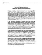
An interesting topic for discussion, that highlights differences in our theories of aggregate supply is that of anti-cyclical vs. pro-cyclical wages. Lucas’s aggregate supply function (shown earlier) shows how output will fluctuate depending on the scale of the “price surprise”. This is also true for wages and so wages (w) can be substituted into the equation in place of price (p). When we look at the aggregate supply function in this way we see that if the real wage rises then output will also rise. If we take wage data from the U.S between 1960 and 2000 and plot real wages against the percentage change in real GDP we observe that as output fluctuates, the real wage typically moves in the same direction. From this we can see that in reality, wages are procyclical which is consistent with the predictions of Lucas’s model. However, this does not agree with the sticky wage model, which predicts that the real wage fluctuates in the opposite direction from employment and output. Thus, the sticky wage model does not fully explain the AS curve. Models in which the labour demand curve shifts over the business cycle are favoured by most economists. In the sticky wage model we merely observe workers moving up and down the labour demand curve. Anti cyclical wages is a large implication of models based on the labour market.

An essential process of formulating and critically assessing different theories is actually testing the models to give results from the real world. This allows us to compare what theories predict and how those predictions hold up in the face of real results. As stated earlier, the model predicts that government policy can only be effective when it creates a price surprise. When agents form expectations rationally they have all available information, including that of the money supply process. Lucas carried out empirical testing of his model by taking nominal and real GDP data from around 50 countries and running a regression of:

Yt = α0 + α1 t + α2 y t-1 + τΔ xt

When plotting the coefficient of the price surprise against the variability of aggregate demand, Lucas found that his estimate of τ alone was sufficient in explaining the price surprise.

Later empirical work by Barro involved using time series data from the U.S. His work involved splitting the money supply into 2 components, predictable variables and unpredictable variables. He then proceeded to run two regressions with unemployment (in natural log form) as the dependent variable firstly against known (predictable) variables in the economy, e.g. government deficit, and then against unknown (unpredictable) variables. By doing this Barro hoped to find the significance of predictable values and unpredictable values on output. From the F test results from each regression, he found that predictable values were statistically insignificant while the unpredictable variables in explaining output were statistically significant. Mishkin argued that Barro’s methods were unsuitable for this work, saying that the tests should have been carried out as one large regression rather than two separate regressions.

Both Lucas’s and Barro’s tests concluded the policy ineffectiveness proposition that a systematic policy cannot affect real variables. However, science does not stop still and further studies from other researchers have found real responses from systematic policy. There are several viewpoints on the validity of the tests on this model. Mishkin argues that Lucas’ findings are correct but disapproves of Barro’s work. Yet Mankiw and Ball approve of Barro’s work and disapprove of Lucas’s.

In conclusion it is important to say that not all rational expectations models give the policy ineffectiveness result. Real variables can still be affected in a model with rational expectations when for example, the monetary authority has superior information to agents. In a general conclusion of the 3 aggregate supply theories, my personal favourite is the sticky price model. It’s assumptions are more plausible and realistic in relation to some of the far fetched visions of reality that the imperfect information model assumes.