- A camera with lens and viewing screen.
- Double wedge aerofoil, where t/c=0.08 and has a wedge angle of 10.5º.
- Plint TE25/A Supersonic wind tunnel, with a test section of width 25mm, and 25 pressure tappings across its convergent and divergent sections. See Figure 3 and Table 1 for positions and spacing’s of tappings.
-
A Pressure tap connected in the contraction section to measure stagnation pressure. This will be referred to as P26.
-
Two pressure tappings are placed above aerofoil at ¼ chord and ¾ chord (at the centre of each linear section), and these are P27 and P28 respectively. These measure the upstream pressure.
- Computer with appropriate software installed, to record and capture experimental data. All pressure tappings are connected to computer via a transducer.
Figure 2 – Schlieren system and setup
Figure 3 – Pressure Tap positions along wind tunnel.
Experimental Procedure
The rig operator gradually opened the injector valve and adjusted its opening so that a steady rate is maintained for a couple of minutes. During the steady-state time the pressure levels were read from the computer. The outputs are converted into mm of Mercury (Hg). The pressure does not change for all conditions upstream the aerofoil leading edge, due to the nature of propagation of disturbances in supersonic flows.
The operation was repeated for angle of attacks 0º, 2º, -2º, 4º, -4º, 5.25º, -5.25º, 8º, -8º. The reason that the operation was repeated for the corresponding negative AOA was to record the downstream pressure on the aerofoil, because the aerofoil is symmetrical when set to negative α the upstream pressure is equal to the downstream pressure of when the same value of α is positive.
Results
Pressure Tap Readings
Table 1 – Geometrical details of nozzle and pressure tapping positions and their corresponding experimental values for positive angle of attack.
Table 2 - Geometrical details of nozzle and pressure tapping positions and their corresponding experimental values for negative angle of attack.
Table 3 – P26, P27, and P28 experimental values recorded
for each angle of attack
Schlieren Images
For α = 0°
For α = 2° For α = -2°
For α = 4° For α = -4°
For α = 5.25° For α = -5.25°
For α = 8° For α = -8°
Theory and Calculations
Mach number and Pressure Ratio
To calculate free stream pressure, P∞, use equation (1):
Where M∞=1.8, γ=1.4, and Po=P26+Pat
To calculate the experimental mach numbers, substitute the absolute pressure, P, from Table 1, for P∞:
Rearrange to get M:
Table A1 in the Appendix shows the calculated Experimental Mach numbers and Pressure ratios.
The Theoretical values of Mach numbers and Pressure ratios can be obtained using Appendix A and B from “Fundamentals of Aerodynamics” by Anderson, and using the cross sectional area ratio from Table 1. See Table A2 in the Appendix for values.
The following graphs plot the values found above:
Graph 1 – Mach number variation Vs x (distance of pressure taps)
Graph 2 – Mach number variation Vs A/A* (cross sectional area ratio)
Graph 3 – Ratio of stagnation static pressure to stagnation pressure Vs x (mm)
Lift and Drag Coefficients
To calculate experimental Lift and Drag coefficients first the pressure coefficients have to be calculated, using equation (3) and the values from Table 3:
, where P = Pman + Pat, and M∞ = 1.8
Then calculate the corresponding normal and parallel force coefficients using equations (4) & (5):
Where t/c = 0.08
Then using equations (6) & (7), the experimental Lift and Drag coefficients can be obtained.
To calculate the theoretical Lift and Drag coefficients for each angle of attack, use equations (8) & (9):
All the above calculated values are in the Appendix, Tables A3-A8
The following graphs plot the values calculated using the above.
Graph 4 – CL Vs angle of attack
Graph 5 – CD Vs angle of attack
Graph 6 – CL Vs CL
Discussion
Graph 1 shows the distribution of the Mach number across the wind tunnel. As you can see from the graph that the theoretical and experimental Mach number are very close together. The drop in the experimental Mach number for is due to the reduction in the pressure in the compressor. Also the graph scatters after 450mm this could be the due to turbulence after the test section.
Graph 2 is just the Mach number variation against the area ratio.
Graph 3 shows the relationship between pressure ratio and x, as you can see that again the experimental and theoretical values are very close together, this indicates that the experiment was quite accurate for most of the pressure tappings.
For the above three graphs mentioned, I have noticed that when x is about 200mm the experimental values deviate and then return back towards the theoretical, and by looking at that position in the divergent part of the tunnel I cant conclude any phenomena at this position therefore it only suggests that this pressure tap is slightly defective or has a loose connection.
Graph 4 shows that, theoretically CL increases linearly as AOA increases (given that AOA is less than stall angle), but the experimental values are very similar to the theoretical but after 5o, there is a sharp rise in the gradient of the line, and a CL value increases by up 50%.
This trend is also for true for graph 5 and 6.
The Schlieren images show that up to 4 degrees the oblique shock wave is ordinary, but after this there is a reflection shock wave appearing in the image this due to the larger angle created by the AOA and the wedge angle against the flow, and consequently creates a larger oblique shock angle.
Conclusion
The main purpose of this lab was to find out any changes occurred in the aerodynamic properties before and after shock waves.
I felt that this experiment was highly educational and gave me a good understanding of how the aerodynamic properties are affected in supersonic flow.
If I were to repeat the experiment again I would attach two pressure taps below the aerofoil so that negative AOA runs didn’t have to be carried out, but more importantly the majority of test sections are not symmetrical therefore that method cannot be used.
References
- Fundamentals of Aerodynamics, by Anderson
- Laboratory handout, By Dr Filippone
Appendix
Tables of Calculations
Table A1 - Experimental Mach numbers and pressure ratios
Table A2 - Theoretical Mach numbers and Pressure ratios
Table A3 - For α=0°
Table A4 - For α=2°
Table A5 - For α=4°
Table A6 - For α=5.25°
Table A7 - For α=8°
Table A8 – Experimental and Theoretical values for Lift and Drag coefficients
Convergent-Divergent Nozzle Flows
For isentropic flow conditions, the ratio of stagnation pressure to static pressure, Po/P, is a function of the free stream Mach number, M:
(1)
Where γ is the ratio between specific heats, γ=CP/Cv. Assume γ=1.4 as a constant through the experiment.
For flows in a converging-diverging nozzle with sonic conditions at the throat, the Mach number distribution within the nozzle is related to the cross sectional area distribution, A/A*, through the Area-Mach number relation:
(2)
Supersonic Aerofoil Flow
The double wedge Aerofoil is characterised by its wedge angle and maximum thickness. From one datum we can derive the other. The two dimensional surface pressure coefficient is defined as:
(3)
The normal and parallel force coefficients on the aerofoil can be computed from:
(4)
(5)
Where CP1 is derived from the ‘27 upper’ values
CP2 is derived from the ‘28 upper’ values
CP3 is derived from the ‘27 lower’ values
CP4 is derived from the ‘28 lower’ values
The calculation of lift and wave drag can be done by decomposing the normal and axial forces into forces normal and axial to the free stream:
(6)
(7)
Theoretical Lift and Drag Coefficients
The inviscid supersonic flow around an aerofoil can be predicted with a fairly good approximation using the linearised flow theory of the flow equations (Ackeret, 1929). The theory is limited to thin aerofoils and small angles of attack (e.g. small perturbations to the flow field). The results of the Ackeret’s theory are given below:
(8)
(9)
Where α is in radians.
Figure 4 – Shock system on a double wedge aerofoil