Laboratory Report
E405 Mechanics of Fluids
CALIBRATION OF AN OPEN CIRCUIT WIND TUNNEL
Name:
Personal Tutor:
Tutor
Note:
L
Results
The results have been recorded and are present on the tables below. The initial recorded data has been converted to more suitable units, to avoid confusion and to progress into further calculations. For any units which were inches/H20 will be converted into mm/H20. Also when conducting this experiment the instruments were inclined at a certain angle, Thus when converting it the vertical component was also calculated into consideration.
Table of Results:
Table A
Table 1
Here the velocity ratio is constant. The coefficients are calculate by there formulae which is in the handout. The Data is also shown on the graph figure 3.

Figure 3
The velocity and the Static, Stagnation coefficients all follow a similar pattern.
Table 2:
Figure 4:
At the initial part of the Graph there is a dip due to the turbulence of the fan. It takes a short amount of time for the readings that are necessary to be available.
Discussion
Assessment of uncertainty
Experimental error is typically a function of random errors and systematic errors. There were many sources of uncertainty in the experiment. Random error could have been ...
This is a preview of the whole essay
Figure 3
The velocity and the Static, Stagnation coefficients all follow a similar pattern.
Table 2:
Figure 4:
At the initial part of the Graph there is a dip due to the turbulence of the fan. It takes a short amount of time for the readings that are necessary to be available.
Discussion
Assessment of uncertainty
Experimental error is typically a function of random errors and systematic errors. There were many sources of uncertainty in the experiment. Random error could have been avoided from the start if there were a larger sample size of data, thus avoiding any anomalous results. The systematic errors mainly occurred due to the instrumentation.
All of the instrumentation used had an error value:
Multi tube slope reservoir: ±0.05 inches
Sloped Monometers: ±0.5mm
At the start of the experiment there may have been a systematic uncertainty in the readings due to the fact that the experiment had already been conducted before. This may have lead to readings not being exactly on their zero mark, thus affecting our readings and values for the coefficients completely.
The Pitot Static tube was placed at the centreline of the working section and was correctly aligned before every reading; however the quality of the instrument was not assessed. If it were blocked or slightly damaged this would have a direct impact on the values of static and stagnation pressure recorded. In reality the flow through the working section is not always constant, when recording data with Pitot static tube from the centre to the left it was assumed the readings would be symmetrical for the right, producing predictions which may be false when perceiving the flow in a realistic approach.
The multi tube slope reservoir manometer was also a key instrument as we used it to obtain significant data; it was inclined at an angle where it would be easier to read the measurements. The manometers had to be checked so that they were all levelled. Because the points had to be visually read off of a manometer scale and verbally transferred to the data recorder, there was a high probability of a mistake. The instrument is just as good as the person who is reading it as it depends on the human eye’s ability to interpret small graduations, this could result in human error. Also when recording the data, it was scaled up from inches to millimetres. Using millimetres as the ideal measuring unit on the instrument would allow it to be more accurate since there would be finer divisions. This would allow a person to see more vividly if there were small changes when recording the data. Also any errors present in the values measured for static and stagnation pressures would be magnified in the calculation of coefficients.
Discussion of results
There was a great influence in the symmetry of the experimental setup and with the results. For example when conducting the experiment the Pitot static tube was measured at the centre line of the working section. It was then moved left after every reading. The readings for the left side of the working section were assumed to be the same as the right side of the working section. The main assumption towards this was that the working section was symmetrical. This seemed to be reasonable as the pressures remained roughly constant. There is also a slight depiction of this in figure 4. At the start, the static gradient coefficient starts to increase steadily rather than have an immediate constant value. It was due to the turbulence within the system. At the end of this graph it seems that the Static gradient coefficient dramatically decreased. However the data did not make sense as the pressure decreased with the cross-section. It was actually due to the fan’s presence in the wind tunnel as it interrupts the airflow. While this occurred the cross-sectional area did the exact opposite, it decreased with the increment for the position of the whole.
Reading tables A and table 1 the airflow through the wind tunnel’s working section was very uniform. The Variation in stagnation and static pressure were near-constant, there was only slight increases between the two. The velocity ratio was also shown as a constant value. Table 1 and figure 3 proves this occurs as all the values incline towards the value 1. Also in figure 3 the centre line is represented by the origin of the graph.
The experiment also held for the validity of Bernoulli’s equation. Bernoulli's principle states that for an , an increase in the speed of the fluid occurs simultaneously with a decrease in or a decrease in the 's .
The assumptions for the Bernoulli equation are:
- Steady State flow
- Incompressible flow
- The flow is along a streamline
- Inviscid flow
However air is a compressible flow, the assumption is wrong, this is actually shown in table 1 where the cross-sectional area decreases from 1.634m2 to 0.347m2. The Air must compress around the tunnel. How can this still show the validity of Bernoulli’s equation?
An incompressible flow is a fluid motion with negligible changes in density. No fluid is truly incompressible, since even liquids can have their density increased through application of sufficient pressure. But density changes in a flow will be negligible if the Mach number, Ma, of the flow is small. This condition for incompressible flow is given by the equation below,
Where V is the fluid velocity and a is the speed of sound of the fluid. It is nearly impossible to attain Ma = 0.3 in liquid flow because of the very high pressures required. Thus in this case the air flow can be represented as an incompressible flow.
When recording data, the static and stagnation pressures had to be converted to mm/H20, represented in the table of results. The readings were taken at certain time intervals, if there were shorter time intervals there may have been moments were a finer progression of the pressure rather than a sudden increase of data would be achieved. However the pressures would still be overall a constant value, indicating that this was a steady state flow, independent of time.
Saadat Sabur