A load of 1kg
Two clock gauges on magnetic stands used to measure the free end horizontal and vertical deflections.
4. Methodology
The dimensions of the cross section of the beam were carefully measured twice using callipers. The average of each dimension was then taken. These were used in the calculation of the theoretical position of the centroid and angle of principal axis using the formulae in section 2. The dimensions are shown in figure 4.
Experimental procedure:
In order to experimentally determine the position of the principal axis, three individuals were required to carry out the following tasks:
One to rotate the beam
One to load the free end and take the deflection readings on the clock gauges
One to record these readings
This was repeated every 10⁰ increment from 0⁰ to 180⁰. The resulting data and graphs are shown in section 5.
5. Results
5.1 Experimental results
Table 1
Graph 1 shows the variation of horizontal and vertical deflections with the angle ϕ rotated. Trend lines were drawn to show the trend that the discrete points follow, which appears to approximate to a sine curve for δv and a cosine curve δh. To estimate the value of the principle angle, vertical lines were drawn at the points where δh =0, i.e. where it crosses the x-axis. By inspection these were found to be:
ϕ1= 37⁰ and ϕ2= 120⁰.
5.2 Theoretical results
By using equations 1,2,3,4 it was found that:
ϕ1=33.096⁰ and ϕ2=123.096⁰
6 Analysis of results
Table 1 shows the variation of horizontal and vertical deflections with the angle of rotation, ϕ, when a load of 1kg is applied at the free end of the cantilever. The resulting graph is shown in graph 1. The angle ϕ1 or ϕ2 at which the horizontal deflection is equal to zero is said to be the principal angle. The graph shows two points at which the value of δH changes sign, and δV becomes a maximum. This is where the angle ϕ for the principle axis occurs. These were determined by simply sketching vertical lines on the graphs at the points where δH crosses the x-axis as shown in page 5. These were then compared with the theoretical values shown in 5.2.
6.1 Calculation of theoretical ϕ1 and ϕ2
Using Matlab ® with equations 1-4 and
analysis of figure 5
It was found that (to 2dp):
Ixx = 269836.21mm4
Iyy =161776.95 mm4
Ixy = -122456.42 mm4
ϕ1=33.096⁰ and ϕ2=123.096⁰
6.2 Comparison
The experimental value of ϕ1 is 4⁰ larger than the theoretical value. In turn the experimental value of ϕ2 approximately 3⁰ less than the theoretical value. This discrepancy is owed to experimental errors which are discussed in 6.3.
6.3 Error Analysis
Measurement error
The error in the instrumentation is given as half the smallest division plus human error (where appropriate).
Error in callipers: 0.5 × 0.01mm = ± 0.005mm
Error in clock gauges: 0.5 × 0.1mm =± 0.05mm
Error in protractor: 0.5×1⁰ + 1⁰ (Human error) = ±1.5⁰
The error in the protractor would contribute to the error in the measured values of ϕ1 and ϕ2. Their relative error can be calculated as:
= (δϕ1 measured)
= (δϕ2 measured)
The error in the clock gauges would contribute to the errors in the deflections. These are shown in table 1.
Error in theoretical ϕ1 and ϕ2
The measurement error in the callipers would affect the accuracy of the theoretical values of ϕ1 and ϕ2. However estimating their error using conventional partial derivatives would be complex and unnecessary. The error of this was calculated using the maximum and minimum values of the dimension of the cross section to find the error in ϕ, δϕ. This was done using the Matlab script.
Note that the b1, b2, d1, d2 are averages of two readings respectively. Therefore the resulting error is 0.005 + 0.005 = ±0.01mm .
b1 = 50.77 ± 0.01mm
d1 = 6.76 ± 0.01mm
b2 = 6.7 ± 0.01mm
d2 = 62.27± 0.01mm
Using maximum b’s and d’s:
ϕ1 max = 33.0967⁰
Using minimum b’s and d’s
ϕ1 min = 32.9884⁰
We know ϕ1 = 33.0961
Therefore:
δϕ =
δϕ= ± 0.0542⁰ Therefore
ϕ1 = 33.0961±0.0542⁰
ϕ2 =123.0961± 0.0542⁰
7 Discussion
The pattern described by δh and δv shows approximately cosine and sine curves (Graph1). The points where δh crosses the x-axis corresponds to the points where δv is a maximum. The corresponding values of ϕ at these points are said to be the principle angles of the principle plane. The experimental results show the values of angles of principle plane as 37⁰ and 120⁰. Whereas the theoretical values show corresponding values of approximately 33.1⁰ and 123.1⁰. This shows a difference of 4.1⁰ and 3.1⁰ respectively. This discrepancy is owed to a combination of factors, namely the measurement error (6.3) and Human error (7.1). The human error consists of quantifiable and non-quantifiable contributors. The quantifiable involves the measurement of the angle ϕ and the non-quantifiable includes possible leaning on the table on which the apparatus was mounted. Human error is discussed further in 7.1.
7.1 Human error
The measured values of ϕ1 and ϕ2 are derived from estimating that δv and δh follow the trend line described in graph 1. However, the pattern of the discrete values does not perfectly describe a sine and cosine curve. This can be owed to human error. Such error could have been encountered when the beam was being adjusted to the correct angle. Turning the beam by such a small angle required a firm hand to accurately adjust the beam. This resulted in a reading error of ±1⁰ off the target. This problem could be rectified by using a lever to rotate the bearing rather than bare hands.
Any leaning or vibration on the table upon which the apparatus was mounted could have affected the readings on the clock gauges. This could have been avoided by not making contact with the table whist readings are being taken.
8 Conclusions
Despite the discrepancies that can easily be seen in the graph 1, the results from the measured values showed a reasonably close agreement with the theoretical values;
ϕ1(measured) : 37⁰, ϕ1(theoretical):33.1⁰ showing a 4.1⁰ difference.
ϕ2(measured): 120⁰,ϕ2(theoretical ):123.1⁰ showing 3.1⁰ difference.
In order to reduce these errors, the experiment could have been repeated several times using small increments of ϕ, say 1⁰. This would achieve smoother graphs for δh and δv from which more accurate values of ϕ could be found by eye with the aid of a suitable trend-line and appropriate vertical lines .
9 References
Title: ME3 Laboratory, Solid Mechanics, Experiment S1, Unsymmetric Bending Of Beams
Organization: The University Of Edinburgh
10. Appendix
10.1Cross section of beam
10.2 Matlab code
% Calculation of theoretical Phi
% Arelo Tanoh s0805209
% Variable dictionary
% b1 breadth of rectangle 1 (mm)
% d1 depth of rectangle 1 (mm)
% b2 breadth of rectangle 2 (mm)
% d2 depth of rectangle 2 + d1 (62.7) (mm)
% A1 Area of rectangle 1 (mm^2)
% A2 Area of rectangle 2 (mm^2)
% Atotal Total Area of beam cross sectional area (mm^2)
% Xg x coordinate of centroid (mm)
% Yg y coordinate of centroid (mm)
% Ixx second moment of area about x-axis (mm^4)
% Iyy second moment of area about y-axis (mm^4)
% Ixy cross moment of area (mm^4)
% Phi1 angle of principle axis (degrees)
% Phi2 angle of principle axis (degrees)
% input dimensions
b1 = input('enter b1 : ');
d1 = input('enter d1 : ');
b2 = input('enter b2 : ');
d2 = input('enter d2 : ');
% calculate areas
A1 = b1*d1;
A2 = b2*(d2-d1);
% Total Area
Atotal = A1 + A2;
% First Moment
Xg = (A1*b1/2 + A2*(b2/2))/Atotal;
Yg = ((A1*d1/2 + A2*(d1 + (d2-d1)/2 )))/Atotal;
% Second Moment
Ix1 = ( (b1*d1^3)/12 + A1*(d1/2 - Yg)^2 );
Ix2 = ( (b2*(d2-d1)^3)/12 + A2*((d1+(d2-d1)/2)-Yg)^2);
Ixx = Ix1 + Ix2;
% using equation 3
Iy1 = ( (d1*b1^3)/12 + A1*(b1/2 - Xg)^2);
Iy2 = ( ((d2-d1)*b2^3)/12 + A2*(b2/2 - Xg)^2);
Iyy = Iy1 + Iy2;
% Cross moment using equation 4
Ix1y1 = A1*(b1/2 - Xg)*(-1*(Yg - d1/2));
Ix2y2 = A2*(-1*(Xg - b2/2)*(((d2-d1)/2 + d1) - Yg));
Ixy = Ix1y1 + Ix2y2;
% Angle Phi using equation 1
phi = 0.5*atand(-2*Ixy/(Ixx - Iyy)) ;
phi2 = phi + 90;
% display results
disp(['Xgis' num2str(Xg) 'mm']);
disp(['Yg is' num2str(Yg) 'mm']);
disp(['Ixx is' num2str(Ixx) 'mm^4']);
disp(['Iyy is' num2str(Iyy) 'mm^4']);
disp(['Ixy is' num2str(Ixy) 'mm^4']);
disp(['Phi 1 is' num2str(phi) 'degrees']);
disp(['Phi 2 is' num2str(phi2) 'degrees']);
10.3 Sample Output of code
enter b1 (mm) : 50.77
enter d1 (mm) : 6.76
enter b2(mm) : 6.7
enter d2(mm) : 62.27
Xg is 13.9252 mm
Yg is 19.5725 mm
Ixx is 269836.2125 mm^4
Iyy is 161776.952 mm^4
Ixy is -122456.4187 mm^4
Phi 1 is 33.0961 degrees
Phi 2 is 123.0961 degrees