Each point on the LM curve reflects a particular equilibrium situation in the money market equilibrium diagram, based on a particular level of income. In the money market equilibrium diagram, the function is simply the willingness to hold cash balances instead of . For this function, the nominal interest rate (on the vertical axis) is plotted against the quantity of cash balances (or liquidity), on the horizontal. The liquidity preference function is downward sloping. Two basic elements determine the quantity of cash balances demanded (liquidity preference) and therefore the position and slope of the function:
1) Transactions demand for money: this includes both (a) the willingness to hold cash for everyday transactions and (b) a precautionary measure (money demand in case of emergencies). Transactions demand is positively related to real GDP (represented by Y,and also referred to as income). This is simply explained - as GDP increases, so does spending and therefore transactions. As GDP is considered exogenous to the liquidity preference function, changes in GDP shift the curve. For example, an increase in GDP will, , move the entire liquidity preference function rightward in response to the GDP increase.
2) Speculative demand for money: this is the willingness to hold cash instead of securities as an asset for investment purposes. Speculative demand is inversely related to the interest rate. As the interest rate rises, the of holding cash increases - the incentive will be to move into securities.
General Market:
General equilibrium theory is a branch of theoretical . It seeks to explain the behavior of supply, demand, and prices in a whole economy with several or many interacting markets, by seeking to prove that a set of prices exists that will result in an overall equilibrium, hence general equilibrium, in contrast to , which only analyzes single markets. As with all models, this is an abstraction from a real economy; it is proposed as being a useful model, both by considering equilibrium prices as long-term prices and by considering actual prices as deviations from equilibrium.
It is often assumed that agents are , and under that assumption two common notions of equilibrium exist: Walrasian (or ) equilibrium, and its generalization; a price equilibrium with transfers.
Broadly speaking, general equilibrium tries to give an understanding of the whole economy using a "bottom-up" approach, starting with individual markets and agents. , as developed by the , focused on a "top-down" approach, where the analysis starts with larger aggregates, the "big picture". Therefore, general equilibrium theory has traditionally been classified as part of .
The difference is not as clear as it used to be, since much of modern macroeconomics has emphasized , and has constructed . General equilibrium macroeconomic models usually have a simplified structure that only incorporates a few markets, like a "goods market" and a "financial market". In contrast, general equilibrium models in the microeconomic tradition typically involve a multitude of different goods markets. They are usually complex and require computers to help with numerical solutions.
In a market system the prices and production of all goods, including the and interest, are interrelated. A change in the price of one good, say bread, may affect another price, such as bakers' wages. If bakers differ in tastes from others, the demand for bread might be affected by a change in bakers' wages, with a consequent effect on the price of bread. Calculating the equilibrium price of just one good, in theory, requires an analysis that accounts for all of the millions of different goods that are available.
National Income Model:
A variety of measures of national income and output are used in to estimate total economic activity in a country or region, including (GDP), gross national product (), and (NNI). All are specially concerned with counting the total amount of goods and services produced within some "boundary". The boundary is usually defined by geography or citizenship, and may also restrict the goods and services that are counted. For instance, some measures count only goods and services that are exchanged for money, excluding bartered goods, while other measures may attempt to include bartered goods by imputing monetary values to them.
In order to count a good or service it is necessary to assign some value to it. The value that the measures of national income and output assign to a good or service is its market value – the price it fetches when bought or sold. The actual usefulness of a product (its use-value) is not measured – assuming the use-value to be any different from its market value.
Three strategies have been used to obtain the market values of all the goods and services produced: the product (or output) method, the expenditure method, and the income method. The product method looks at the economy on an industry-by-industry basis. The total output of the economy is the sum of the outputs of every industry. However, since an output of one industry may be used by another industry and become part of the output of that second industry, to avoid counting the item twice we use not the value output by each industry, but the value-added; that is, the difference between the value of what it puts out and what it takes in. The total value produced by the economy is the sum of the values-added by every industry.
The expenditure method is based on the idea that all products are bought by somebody or some organisation. Therefore we sum up the total amount of money people and organisations spend in buying things. This amount must equal the value of everything produced. Usually expenditures by private individuals, expenditures by businesses, and expenditures by government are calculated separately and then summed to give the total expenditure. Also, a correction term must be introduced to account for imports and exports outside the boundary.
The income method works by summing the incomes of all producers within the boundary. Since what they are paid is just the market value of their product, their total income must be the total value of the product. Wages, proprieter's incomes, and corporate profits are the major subdivisions of income.
Open and Close/ Income and Output Model :
A. Equilibrium
The equilibrium condition around which the model is built is:
Y = C + Id + G + X - M
Remember this means that total demand for national output equals national output. But national absorption (C + Id + G) does not have to equal national output, even in equilibrium, if the economy is open. Equilibrium still means what it did with a closed economy, which is to say that there is no change in inventories. Equilibrium in no way implies trade balance.
We solve for a situation in which domestic investment is exactly at the level of planned purchases of plant and equipment; change in inventories is zero.)
B. Example
C = 10 + .8(Y-T) (Just like the consumption function from the closed economy)
S = -10 + .2(Y - T)
Id = 23
G = 10
T = 10
M = .3Y
X = 15
To find equilibrium Y:
Y = C + Id + G + X - M
Y = 10 + .8(Y - 10) + 23 + 10 + 15 - .3Y
Y = 50 + .5Y
.5Y = 50
Y = 100
Note that at this Y=100, C = 82, + Id = 23, and G = 10 so C + Id + G (or E) = 115.
Check this against trade: if Y=100 then M = 30, while X = 15, so the country is indeed getting more stuff than it makes; in more technical language total absorption (E) exceeds total output by 15, which is the amount of the trade deficit.
This can be seen in the diagram.
C. Thinking about the Example's Solution
At this point we have solved the problem by focusing on goods. The equation
Y = C + Id + G + X - M
draws our attention to the fact that in equilibrium, national income equals aggregate demand.
But we know from the diagrams that the financial flows must match as well.
Note that if Y = 100, S = 8. Note further that Id = 23. Who is financing this gap of 15? Foreigners. And indeed 15 is precisely the observed gap between imports and exports, which has to be made up by such financing. The relevant formula is:
S = Id + If
Remembering that If (a net concept) is negative in this case.
The lower part of the diagram for this section graphs net exports and the gap between savings and domestic investment. Savings is also graphed by itself. Here equilibrium is the point where the amount of financing forthcoming from foreigners is enough to fill the domestic savings-investment gap.
D. Further notes
In this model the level of output (which is also income) adjusts in response to changes in various exogenously-determined components of demand. By assuming that X is exogenous, while M is a function of Y, we get a model that tells us what the resulting If is. In other words the model produces a domestic equilibrium; if the external finance is forthcoming then it's an external equilibrium too. As we just saw, you can solve this model for equilibrium Y either in terms of demand (Y = C + Id + G + X - M) or in terms of the balance of payments (S - Id = If = X - M).
Apart from some practice with the balances, this model provides a useful insight for countries with relatively open economies: any policy that raises income will worsen the trade balance. (Although the model does not show it, higher domestic income may also reduce exports, as some goods that could be exported are sold locally instead.) Note that by assuming that X is exogenous, we are considering a small country case. For a large country, an increase in it imports should raise foreign incomes, and lead to higher exports.
This model assumes that enough foreign finance is always available to cover a trade deficit. Other models do not make that assumption. For example in the open-economy version of the , a model which includes interest rates, a higher domestic interest rate may be required to tempt foreign lenders. Alternatively, a country may find itself limited, or rationed, in the amount of foreign finance it can obtain. That might limit growth.
Application Eigen Vector:
The eigenvectors of a are the non-zero vectors that, after being by the matrix, remain parallel to the original vector. For each eigenvector, the corresponding eigenvalue is the factor by which the eigenvector is scaled when multiplied by the matrix. The prefix is adopted from the word "eigen" for "own" in the sense of a characteristic description. The eigenvectors are sometimes also calledcharacteristic vectors. Similarly, the eigenvalues are also known as characteristic values.
The mathematical expression of this idea is as follows: if A is a square matrix, a non-zero vector v is an eigenvector of A if there is a scalar λ(lambda) such that
The scalar λ (lambda) is said to be the eigen value of A corresponding to v. An eigen space of A is the set of all eigenvectors with the same eigen value together with the . However, the zero vector is not an eigenvector.
These ideas often are extended to more general situations, where scalars are elements of any field, vectors are elements of any vector space, and linear transformations may or may not be represented by matrix multiplication. For example, instead of , scalars may be ; instead of arrows, vectors may be functions or ; instead of matrix multiplication, linear transformations may be operators such as the derivative from . These are only a few of countless examples where eigenvectors and eigen values are important.
In such cases, the concept of direction loses its ordinary meaning, and is given an abstract definition. Even so, if that abstract direction is unchanged by a given linear transformation, the prefix "eigen" is used, as in , , , eigen state, and eigen frequency.
Eigen values and eigenvectors have many applications in both pure and applied mathematics. They are used in , in , and in many other areas.
Surge Function:
The family of surge functions is the family of functions f(t) = Ate
−bt with parameter values A and b both positive. We work with independent variable t here, because we will be thinking about these functions as representing a quantity changing in time. Also we will restrict our view to values of t ≥ 0. Surge functions display an initial linear growth followed by an exponential decay.
They are used in modeling situations where there is an initial input of a substance into a system at a constant rate, followed by an elimination of the substance once the input has ended. For example, the uptake of a drug into the bloodstream followed by the elimination of the drug from the body. (We will examine a particular example below.)
1. To see the “initial linear growth followed by an exponential decay” behavior of the surge functions, graph on Fathom (with t ≥ 0) the following 3 equations with sliders A and b: y = Ate −bt (the surge function)
y = At (linear with slope A)
y = e
−bt
(Exponential decay with decay constant b)
Vary the slider values and discuss the behaviours you observe, particularly the effect of varying each of the sliders A and b individually.
Convex Function and Convex set:
In , a real-valued function f(x) defined on an interval is called convex (or convex downward or concave upward) if the graph of the function lies below the line segment joining any two points of the graph. Equivalently, a function is convex if its epigraph (the set of points on or above the graph of the function) is a . More generally, this definition of convex functions makes sense for functions defined on a convex subset of any .
Convex functions play an important role in many areas of mathematics. They are especially important in the study of problems where they are distinguished by a number of convenient properties. For instance, a (strictly) convex function on an open set has no more than one minimum. Even in infinite-dimensional spaces, under suitable additional hypotheses, convex functions continue to satisfy such properties and, as a result, they are the most well-understood functional in the . In , a convex function applied to the of a is always less or equal to the expected value of the convex function of the random variable. This result, known as underlies many important inequalities (including, for instance, the and ).
8)Bordered Hessian:
A bordered Hessian is used for the second-derivative test in certain constrained optimization problems. Given the function as before:
but adding a constraint function such that:
the bordered Hessian appears as
If there are, say, m constraints then the zero in the north-west corner is an m × m block of zeroes, and there are m border rows at the top and m border columns at the left.
The above rules of positive definite and negative definite can not apply here since a bordered Hessian can not be definite: we have z'Hz = 0 if vector z has a non-zero as its first element, followed by zeroes.
The second derivative test consists here of sign restrictions of the determinants of a certain set of n - m submatrices of the bordered Hessian. Intuitively, think of the m constraints as reducing the problem to one with n - m free variables. (For example, the maximization of f(x1,x2,x3) subject to the constraint x1 + x2 + x3 = 1 can be reduced to the maximization of f(x1,x2,1 − x1 − x2) without constraint).
9) Jacobian Matrices:
In , the Jacobian matrix is the matrix of all first-order of a - or scalar-valued functionwith respect to another vector. Suppose F : Rn → Rm is a function from to Euclidean m-space. Such a function is given by m real-valued component functions, y1(x1,...,xn), ..., ym(x1,...,xn). The partial derivatives of all these functions (if they exist) can be organized in an m-by-n matrix, the Jacobian matrix J of F, as follows:
This matrix is also denoted by and . If (x1,...,xn) are the usual orthogonal Cartesian coordinates, the i th row (i = 1, ..., n) of this matrix corresponds to the of the ith component function yi: . Note that some books define the Jacobian as the transpose of the matrix given above.
The Jacobian determinant (often simply called the Jacobian) is the of the Jacobian matrix (if m = n).