them. This is the equilibrium rate of interest since at this rate, there is no excess supply or excess demand.
Furthermore, if the ecomomy is not at this equilibirum rate, it will get there. If the money market is not in
equilibrium, then people will alter their portfolio assets, and consequently, will alter the interest rate to
(eventually adjusting it to the equilibrium rate). For example, suppose at interest rate r1, the supply of
balances is greater than the demand for them. In such a situation, the holders of these excess balances will
decide to put them into interest bearing acocunts or purchase bonds etc with them, in order to accumulate
some interest on them since otherwise their money is lying about idle. As a result of this increase in
financial investment, the price of such bonds will usually go up, and since financial institutions prefer to pay
lower rates of interest, they will lower the interest rate, eventually bringing it to r*. On the other hand, if the
rate of interest were r2, then the demand for real balances would be greater than the supply of them.
Individuals would therefore have to make withdrawals and sell bonds in order to realize their demand. As a
result, with everyone preoccupied with making withdrawals etc, the banks would have to increase the rate of
interest to attract scarcer funds from savers. With the rate rising, the demand for money balances would
contract, indicated by a movement back up the demand curve.
The LM curve, which shows the combinations of the interest rate and the level of income that are consistent
with equilibrium in the market for real money balances (the "money market), is derived from Keynes' theory
of liquidity preference. To derive it however, we need to add one point about the demand for money
balances.
I said earlier that the demand for money balances depends on the rate of interest. However, it also
depends on the level of income. This makes intuitive sense since an increase in income is going to lead to
an increase in transactions with an increase in transactions inevitably causing an increase in the money
required for them (money is demanded, inter alia, to make transactions). Therefore, an increase in income, is
going to cause an increase in the demand for money balances, which is depicted on our diagram by an
outward shift to the right of the demand curve. As we can then see from the diagram below (a), this causes
an increase in the interest rate from r1 to r2. These changes are then summarized in the LM curve shown in
diagram (b) below.
The LM curve plots the relationship between income and the interest rate. The higher the level of income,
(the higher the demand for transactions and therefore the higher the demand for money balances) the higher
the equilibirum interest rate. (The higher the rate of interest that equilibriates the money market).
Thus we have derived the LM curve under the theory of liquidity preference.
a. An increase in the price level
As noted earlier, the price level is an exogenous variable in the IS-LM model. However, it affects the supply
of money balances. An increase in the price level has the affect of lowering purchasing power, and
consequently, it reduces the amount of real money balances supplied. In the diagram below (a), this is
depicted by a shift to the left of the supply curve for real money balances. Diagram (b) shows what happens
to the LM curve:
Income does not change in this situation. What does happen is that the increase in prices, leading to a fall
in the supply of real balances, causes the interest rate to rise. This means that, at any level of income, a
higher rate of interest is required to equilibriate the money market. This is depicted on the LM curve, by an
upward shift.
b. An increase in the money supply
The money supply is the other exogenous variable in the theory of liquidity preference. Indeed, as it will be
shown below, an increase in the money supply will have the opposite effect to the increase in prices. An
increase in the money supply, ceteris paribus, will increase the quantity of real money balances supplied.
This is depicted in the following diagram (a) by a shift to the right in the supply of real balances. As a
result, we can see from the diagram, that the equilibium interest rate falls. The changes th the LM curve are
shown on diagram (b):
With the quantity of money supplied increasing, and the level of prices and income remaining the same, the
quantity of real balances suppplied increases too. The result is that the supply curve of real balances shifts
ot the right, lowering the interest rate. This means that, for any given level of income, the interest rate that is
required to equilibriate the money market will be lower, which is depicted by the downward shift in the LM
curve.
c. An increase in disposable income
In the previous two situations, the changes to in exogenous variables meant that the LM curve shifted
upward or downward respectively. However, what would happen if there were an increase in disposable
income (an endogenous variable)?
This question has already been answered above. An increase in income will lead to an increase in
transactions which would lead to an increase in the demand for real money balances. The diagrams for this
have already been drawn (see page ). Since the LM curve plots the relationship between income and
interest rate, the effect of an increase in income on the LM curve is simply an extension along the LM curve
(shown in diagram (b) on page )
Does the LM curve depend on the real or the nominal rate of interest?
In deriving the LM curve, under the theory of liquidity preference, I said that Keynes posited that the
demand for money (balances) depends on the rate of interest. However, which rate? The nominal or the real
rate?
The real interest rate is the rate of interest that takes into account purchasing power. In other
words, the real interest rate takes into account inflation, as opposed to the nominal rate of interest which
does not. The real rate of interest is the difference between the nominal interest rate and the rate of inflation.
This relationship is summarized in the following equation:
r = i - *
where r denotes the real rate of interest, i denotes the nominal rate of interest, and * denotes the rate of
inflation.
It seems, prima facie, that the interest rate we are concerned with in deriving the LM relation is the
nominal rate of interest. This is because, the money demand function depedns on the nominal rate of
interest. As mentioned above, when we decide how much money to hold, we take into account the
opportunity cost of holding money rather than financial investment. Money pays a zero nominal interest
rate, whereas bonds (or savings accounts etc) pay a nominal interest rate of i. Hence, the opportunity cost
of holding money is just the difference between the two interest rates, i - 0 = i, which is just the nominal
interest rate. Therefore, money demand depends on the nominal interest rate.
However, in the IS-LM, which is a short run model, where we assume are nominal rigidities, in this
context, sticky prices. Therefore, in IS-LM there is no inflation since the price level is fixed. Recall that the
equation for the real rate of interest is:
r = i - *, and therefore,
i = r + *
However, in IS-LM (short-run) there is no * due to the sticky prices. Therefore, if *=0, then;
i = r + 0 ==> i = r
the nominal rate of interest is equivalent to the real rate of interest, and we can therefore say that the LM
curve depends on the real rate of interest.