The function which I thought modelled the behaviour of the graph is the polynomial quadratic function, because it is clear that the graph has a similar shape to a parabola shape. The equation for the polynomial quadratic function is:
y = ax2 + bx + c
For this equation, I need to find the values for the three unknown variables: a, b and c.
The line of symmetry for this equation is x=5 as:
x = = 5
If the value for x is 3, the value for y is 15.7, based on the data from the original table. Therefore:
15.7 = a(3)2 + b(3) + c
15.7 = 9a + 3b + c
If the value for x is 17, the value for y is 20.85. Therefore:
20.85 = a(17)2 + b(17) + c
20.85 = 289a + 17b + c
I can use simultaneous equations to find the values of a, b and c. First, I will substitute the first equation I found (line of symmetry equation) into the second equation.
15.7 = 9a + 3(-10a) + c
15.7 = -21a + c
Next I will substitute the first equation into the third equation.
20.85 = 289a + 17(-10a) + c
20.85 = 289a – 170a + c
20.85 = 119a + c
To use simultaneous equations:
20.85 = 119a + c
-
15.7 = -21a + c
=
5.15 = 140a
In order to find a:
a= = 0.0368 (to 3 s.f.)
If we substitute this equation into the first equation:
b = -10a = -10(0.0368) = 0.368
Therefore, if we substitute this to the full equation:
20.85 = 119(0.0368) + c
c = 16.47
Therefore, the quadratic equation is:
y = 0.368x2 – 0.368x + 16.47
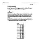
Using information from the equation y= 0.368x2 – 0.368x + 16.47, I put all the new y values in a table (shown below). To compare the values, I plotted the original graph and the function equation on the same set of axes.
In the above graphs, the pink line represents the original equation, and the green line represents the polynomial quadratic function equation.
The above graphs show that while the polynomial quadratic function is quite similar to the original equation, there are some differences. It becomes clear in the first graph (which shows a more closely zoomed-in graph) that the y value of the original equation begins to decrease as the x value moves towards 20. However, the y value of the polynomial quadratic function continues to increase as the x value moves towards 20. The second graph shows this more clearly, and it also shows how the original equation behaves completely differently to the polynomial quadratic function before reaching X=0.
Therefore, the original equation seems to resemble a cubic polynomial more closely than a quadratic equation. For this reason, I decided to use the cubic polynomial function to represent this data. The equation for this function can be calculated from the graph:
y = -0.0041x3 + 0.154x2 – 1.28x + 18.27
The similarity between the original equation and the cubic polynomial equation can be seen in the graphs below:
In the above graphs, the pink line represents the original equation, and the blue line represents the cubic polynomial function equation.
The graph below shows the original equation in pink, the polynomial quadratic function equation in green and the cubic polynomial function equation in blue. This graph acts as a good comparison between the three, and it also allows limitation of the two functions to be found.
In the polynomial quadratic function equation, the shape of the plotted points are close to accurate, but the trend for the rest of the line does not fit. In cubic polynomial function equation, the shape of the plotted points are even closer to accurate, and the trend for the rest of the line is much closer to that of the original equation, but still the line does not fit.
However, any future estimations cannot be based on either of these two models as they do not fit what the natural trend should show. Therefore, the final function I have decided to show is the quartic function (also known as a biquadratic function). The equation for this function can be calculated from the graph:
y = 9.73E-005x4 – 0.00835x3 + 0.217x2 – 1.630x + 18.86
This function can be used to estimate the BMI of a 30-year-old woman in the US.
As shown on the graph above, the BMI for a 30-year-old woman in the US would be 18.62. This value is unreasonable because this is in the same BMI bracket as 12-13 year olds. The median BMI for a 30-year-old woman would not be in the bracket because their height should but much higher than that of a 12-13 year old and their weight should be higher. I would expect the BMI of a 30-year-old woman to be above 21.65, which is the median BMI for a 20-year-old.
Conclusion
While I did manage to find some functions that resembled the original equation, they were all deeply flawed. As previously mentioned, in the polynomial quadratic function equation, the shape of the plotted points are close to accurate, but the trend for the rest of the line does not fit at all. This makes using this function to predict future results impossible. In the cubic polynomial function equation, the shape of the plotted points are even closer to accurate than the polynomial quadratic function equation, and the trend for the rest of the line is much closer to that of the original equation, but still the line does not fit. The quartic function modelled the behaviour of the graph best, but it is only accurate and therefore reasonable up to the age of 20. We see that after reaching 20 on the x-axes, the graph descends to the point where the BMI would be completely impossible for that age group.
I tried many other functions, but could find none that were closer and therefore none that solved this problem.