To find the three unknowns a, b, and c using the matrix method, three equations must be formed. This will be achieved by choosing three guides and their respective distances, and then substituting them into the equation, in place of a, b, and c. The chosen points are the first and last guides and their corresponding distances, (1, 10) and (8, 149) respectively. This is an obvious choice since the fishing line must go through the first and last guides to function properly. For the third equation it would be appropriate to use the median, however since we have eight data points the median would be the fourth and fifth point combined and then divided by 2. This would not be an acceptable course of action since this would result in a point that is not part of the data we are provided with and would result in further inaccuracy. Therefore, for the third equation the fifth point (5, 74) was chosen on the grounds that, between points four and five, it was closest to the mean of 70.625.
Thus, the points are: (1, 10), (5, 74), (8, 149) in the form (x, y).
These numbers will now be substituted into three quadratic equations:
y=ax2+bx+c
Equation 1: 10 = a(1) + b(1) + c
Equation 2: 74 = a(25) + b(5) + c
Equation 3: 149 = a(64) + b(8) + c
Once the above system of equations is formed it is possible to translate them into the following matrices:
A=, Y=, B=
Matrix A represents the values of the chosen guides in the quadratic equations, matrix Y represents the unknown constants, and matrix B represents the placement distance for each of the chosen guides. Using the three matrixes it is possible to form the following matrix equation:
AY=B
=
Now it is possible to use the following matrix property to find the unknowns:
A-1AY=A-1B
IY=A-1B
Y=A-1B
By multiplying A and B with A-1 it is possible to isolate Y; since a matrix multiplied by its inverse becomes an identity matrix (A-1A=I) and IY=Y. Hence, we can find the unknowns.
Which would take the following form for the given values:
=
Using the GDC we are able to obtain the following:
=
Therefore, a≈1.29, b≈8.29, and c≈0.429, to 3 significant figures. By substituting these values into the general expression of the quadratic equation, it is possible to formulate the following quadratic model for Leo’s fishing rod:
y ≈ 1.29x2+8.29x+0.429
OR
ƒ(x) ≈ 1.29x2+8.29x+0.429
The comparison of the quadratic model function with the original data points can be seen in Graph 2.
The same matrix method can be used to formulate a cubic model. The only difference is that the general expression for a cubic function takes the form:
g(x) = ax3+bx2+cx+d
Where g(x)=y.
We can see that in the cubic function above there are four unknowns, a, b, c, and d; thus, requiring that the system of equations consists of four equations rather than three, like we saw in the quadratic model above.
The four guides chosen are one, three, five, and eight. Which form the points (1,10), (3,38), (5,74) and (8,149), respectively.
Equation 1: 10 = a(1) + b(1) + c(1) + d
Equation 2: 38 = a(27) + b(9) + c(3) + d
Equation 3: 74 = a(125) + b(25) + c(5) + d
Equation 4: 149 = a(512) + b(64) + c(8) + d
These equations will form the following matrix equation:
AY=B
Using the same method as before, we can arrive at the following equality:
Using the GDC we are able to find the following values:
By approximating, to three significant digits, the following are the values for the four unknowns: a≈0.0571, b≈0.486, c≈11.3, and d≈ -1.86; resulting in a cubic model function of:
y ≈ 0.0571x3+0.486x2+11.3x-1.86
OR
g(x) ≈ 0.0571x3+0.486x2+11.3x-1.86
The comparison of the cubic model function with the original data points can be seen in Graph 2.
Graph 2. Comparison of quadratic model and cubic model with the original data points
Distance from Tip (cm)
Guide Number (from tip)
From Graph 2, above, it can be seen that the quadratic function only passes through the center of three points making the quadratic model far from a desired model function, and the cubic model passes through the center of four points, making it more accurate than the quadratic model. Generally, the quadratic and cubic models are fairly accurate since they pass through almost all of the points, however neither is the desired function for modeling the optimal placement of guides on a fishing rod because they do not pass through the center of each point. Graph 3 confirms this, as we can see that the quadratic function (f(x)) does not even pass through the 6th and 7th guides, and the cubic function (g(x)) hardly passes through both points.
Graph 3. Zoom-in of points 6 and 7 from Graph 2
Guide Number (from tip)
Distance from Tip (cm)
By analyzing the previous two models we notice that the quadratic model, which has three unknown constant, passes properly through three points and the cubic model, which has four unknown constants passes properly through four points. From this information it can be concluded that if a polynomial function was to be produced to model the optimal placement of guides on a fishing rod, it would have to pass through the centers of all the points. From the above model equations we can also conclude, that for a function to pass through all of the eight points, it would need eight unknowns. Thus, a seventh degree polynomial, with eight unknowns would be perfect. This enables the formation of eight equations that can be solved by the matrix method to result in a model that will pass through all the data points.
The general expression for a seventh degree polynomial is:
h(x)= ax7+bx6+cx5+dx4+ex3+fx2+gx+h
Where, h(x)=y
Equation 1: 10 = a(1)7 +b(1)6 +c(1)5+ d(1)4+ e(1)3 + f(1)2 + g(1) + (1)
Equation 2: 23 = a(2)7 +b(2)6 +c(2)5+ d(2)4+ e(2)3 + f(2)2 + g(2) + (2)
Equation 3: 38 = a(3)7 +b(3)6 +c(3)5+ d(3)4+ e(3)3 + f(3)2 + g (3)+ (3)
Equation 4: 55 = a(4)7 +b(4)6 +c(4)5+ d(4)4+ e(4)3 + f(4)2 + g(4) + (4)
Equation 5: 74 = a(5)7 +b(5)6 +c(5)5+ d(5)4+ e(5)3 + f(5)2 + g (5)+ (5)
Equation 6: 96 = a(6)7 +b(6)6 +c(6)5+ d(6)4+ e(6)3 + f(6)2 + g (6)+ (6)
Equation 7: 120 = a(7)7 +b(7)6 +c(7)5+ d(7)4+ e(7)3 + f(7)2 +g(7) + (7)
Equation 8: 149 = a(8)7 +b(8)6 +c(8)5+ d(8)4+ e(8)3 + f(8)2 +g(8) + (8)
Using the method, above, the resulting matrix equation is:
AY=B
=
Using the GDC, the result is:
=
By substituting the values of Y into the general expression the polynomial model will be:
h(x) ≈ 0.0025793651x7-0.0777777777x6+0.95555552x5–6.152777775x4+22.25138888x3-43.76944443x2+55.79047617x– 18.999999999
And the expression to three significant digits will be:
h(x) ≈ 0.00257x7-0.0778x6+0.9556x5-6.15x4+22.3x3-43.8x2+55.8x-19.0
However, since we are attempting to find the optimal guide placement for the fishing rod, rounding the variables to three significant digits is purposeless since this results in a butterfly effect; where the resulting function will not go through all of the points, as seen below in Graph 3. Therefore we must use the expression without any rounding.
Graph 4. 7th degree polynomial function rounded to 3 sig fig compared to original points
Distance from tip (cm)
Guide Number (from tip)
The seventh degree polynomial function can be seen in Graph 5 below.
Graph 5. Polynomial model compared to original data points
Guide Number (from tip)
Distance from tip (cm)
As seen in Graph 4 the polynomial model goes through the center of all the data points making it the desired function. However, this function does not go through the origin (0,0), the 9th guide at the tip of the fishing rod. This is benign because we have already been provided with the information that there is a ninth guide at the tip of the fishing rod, who’s position does not change; therefore, when figuring out the optimal position for the other guides we can make the assumption that, no matter what, the line will go through the ninth guide.
One other free function that could be used to model the placement of guides on a fishing rod is a quartic function, which takes the form:
k(x) = ax4+bx3+cx2+dx+e
Using the Quartic Regression on the GDC the unknown constants a, b, c, d, and e, are found to be:
Substituting these constants into the general expression, we obtain the following model function:
k(x) ≈ 0.0131x4-0.174x3+1.83x2+8.39x-0.00855
Graph 6. Quartic model function compared to original data points
Guide Number (from tip)
Distance from tip (cm)
The quartic model passes through the centers of five points, so it is more accurate than the quadratic and the cubic model functions. By analyzing the four model functions, it can be concluded that the higher the function is powered, the better it fits the original data of Leo’s fishing rod. As seen from the four graphs of the model functions, the seventh degree polynomial (Graph 5) is the model that fits best since it passes through all the points with out being significantly off from the centers of the points.
To find the quartic function, the Quartic Regression application was used on the GDC. A regression is used to find the line of best fit of a certain set of data. It is possible to compare the quadratic and cubic model functions found using the matrix method with the respective functions found using regressions on the GDC.
Table 2. Comparison of matrix method and regression method
The goal of the comparison between the matrix and regression methods was to show the possibility of error. As seen in Table 2 there is a slight difference between the functions formed using the matrix method and using regressions. The GDC regression method is more precise; therefore we can see that there is error associated with the calculations from the matrix method. This shows that the graphs are slightly inaccurate.
As stated above, the seventh polynomial function best models this situation because it effectively passes through every point of the original data. However, considering real life situations, this model would not be suitable because of its length. The quartic regression model requires fewer variables to solve and it matches the 7th degree polynomial function more accurately than the quadratic and the cubic model functions, as seen in Graph 7 and Graph 8 below.
Graph 7 Quartic regression compared to the polynomial, quadratic and cubic functions
Guide Number (from tip)
Distance from tip (cm)
Graph 8. Quartic regression compared to 7th degree polynomial function
Guide Number (from tip)
Distance from tip (cm)
Therefore, in reality the quartic model function would be most appropriate for modeling the optimal placement of line guides on a fishing rod.
We can also use the quadratic model function to determine the possible placement of the ninth guide, by substituting ‘9’ for x in the model function. As defined before, x is the number of guides and y is the distance from the tip in centimeters.
y=1.29x2+8.29x+0.429
y=1.29(9)2+8.29(9)+0.429
y=179.529
y ≈ 180 cm
Therefore, if a ninth guide was added to the fishing rod it would be approximately 180 cm from the tip. One implication of adding a ninth guide to the fishing rod would be that it could shorten the line and possibly cause difficulty when fishing.
We can further test the quadratic model function by applying it to Mark’s fishing rod, which has a length of 300 cm. The data for Mark’s fishing rod is presented in the table below
Table 3. The number of guides and their respective distances on Mark’s fishing rod
To see how well the quadratic model function fits the data of Mark’s fishing rod see Graph 9.
Graph 9. Quadratic model, ƒ(x)=1.29x2+8.29x+0.429, versus Mark’s fishing rod.
Guide Number (from tip)
Distance from tip (cm)
The quadratic model function does not fit the new data very effectively. It only passes through two points and completely misses the rest, as its exponential increase is greater. In order to understand the changes that are needed to improve the model we can use a quadratic regression on the GDC to find a line of best fit for Mark’s fishing rod.
The result is as follows:
And the improved quadratic model function is:
f(x)=0.935x2+7.72x+2.05
One limitation of the quadratic model is that it only applies to fishing rods similar to Leo’s, as we saw with Mark’s set of data, even though Mark’s fishing rod was not very different. Another limitation of the quadratic model is that the model function must be adjusted every time a guide is added to the fishing rod. According to the new, improved quadratic model function for Mark’s fishing rod, f(x)=0.935x2+7.72x+2.05, if a ninth and tenth guide were added to Mark’s fishing rod, they would be placed 147 cm and 172 cm from the tip, respectively. If we were to create a regression of the data, we would obtain values different from the ones above, the new set of values is below.
The new modified function for Mark’s fishing rod is:
f(x)=0.917x2+7.87x+1.83
Another limitation of the quadratic model is that it does not take into account the length of the fishing rod. A fishing rod with a different length would require more guides, which would result in new data points. Different data points would result in a new curve, which the original model will not fit.