where
Therefore
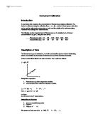
The regression equation is
y - Fluorescence
x - Concentration
The plot of the data is shown below along with its line of best fit the regression line.
Residuals
In the table, we show for each value of , the observed value of together with the predicted or fitted values given by the linear equations. A simple way of assessing the fit of an equation is to calculate the differences between the observed and fitted values. These discrepancies usually termed residuals are also given in the table. Calculating the residual (or error) will represent the unexplained (or residual) variation after fitting a regression model. It is the difference (or left over) between the observed value of the variable and the value suggested by the regression model.
For the model to be a good fit to the data we require the sum of the errors equal zero.
∴
∴
Variance-covariance matrix
∴
The above variance-covariance matrix gives , and
Design matrix
Below is the full fitted model for the data.
Analysis of Variance
The ratiois distributed as F with (1, n –2 ) df.
Here we reject the null hypothesis that β = 0 if the> Fα, 1, n – 2
Rejecting the null hypothesis implies that the variable x influences the variable y. That is the concentration increases as the fluorescence of substance A increases.
Analysis of Variance
Source DF SS MS F P
Regression 1 1003.21 1003.21 2478.53 0.000
Error 4 1.62 0.40
Total 5 1004.83
From the ANOVA table we see that the P-value is 0.000 < 0.01, which is significant at the 1% significance level. We can conclude there is overwhelming evidence to reject the null hypothesis in favour of the alternative hypothesis, i.e. the concentration depends on fluorescence of the substance.
Goodness of fit in regression
Having found the best straight line, the next question is how well it describes the data. We measure this by the fraction
This is called the variance accounted for, symbolised R2. Its square root is the Pearson product-moment correlation coefficient. R2 can vary from 0 (the points are completely random) to 1 (all the points lie exactly on the regression line).
Calculating we find that 99.8% of the data lie on the regression line.
90% Confidence Interval
The 90% confidence interval will be calculated for the unknown parameters α and β, The width of the confidence interval will give us some idea about how uncertain we are about the unknown parameter. A very wide interval may indicate that more data should be collected before anything very definite can be said about the parameter. Confidence intervals are more informative than the simple results of hypothesis tests (where we decide 'reject H0' or 'don't reject H0') since they provide a range of plausible values for the unknown parameter. We will assume the data are collected of independent observations, and are from an underlying normal distribution.
90% Confidence Interval for α
α = 0.90476 ± 2.132 × 0.45771 = (-0.0711, 1.8806)
1.977 < 2.776
∴accept H0 : α = 0.
90% Confidence Interval for β
β = 3.78571 ± 2.132 × 0.07550 = (3.6247, 3.9467)
50.14 > 2.776
∴significant at 5% H0 : β = 0 rejected.
Below is the plot of the 90% confidence interval of the regression line.
90% Prediction Interval about the line at x = 10
Prediction intervals are useful for predicting, for a given X, the Y value of the next experiment. It is used when a fit represents a single experiment, where each Y value is a single observation rather than an average. In this case, the weight for each Y value isn't based upon a standard deviation from multiple observations, but rather is inversely related to the experimental uncertainty for the individual measurement, if such is known. If the uncertainty of the Y measurement is unknown or thought to be equal for all X, all points can use equal 1.0 weights. A 90% prediction interval is the Y range for a given X where there is a 90% probability that the next experiment's Y value will occur, based upon the fit of the present experiment's data.
90% P.I. = 38.76 ± 2.132 × 1.2344 = (36.13, 41.39)
The prediction interval plot for the regression line is shown below.
Re-writing the relationship in the form of
Up to now we have fitted a model of the form , where fluorescence of a substance is determined from the known concentrations. The problem is now reversed where we want to determine the concentration from the known fluorescence level. In order to do this without re-fitting the model, we will simply re-arrange and make the subject of the formula.
When y = 17.5
hence
Having now calculated the value of at a given , we can calculate the associated error.
Given some the predictor is just , the error is given by
Where
hence
= (17.35, 17.65) with 90% confidence.
Conclusion
The regression model fitted for the data is of the form:
where is the dependent variable
is the intercept
is the slope of the regression coefficient
is the independent variable
is the error term.
Where
The regression equation is
The equation will specify the average magnitude of the expected change in Y given a change in X.
Limitations of Regression
An assumption is made with the regression line that it is where it should be.
You cannot assume that the regression line is valid outside the range of the data.
-
You can interpolate, but you cannot extrapolate.
In the model the unknown parameter α and β where calculated. From the 90% confidence interval we know we have a good estimate for the gradient β of the model however more data is required before anything very definite can be said about the intercept of the model the parameter α.