a) t = 9.973
b) t = 19.937
c) t = 39.894
3.
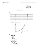
- Table 2:
-
A = )(0.8t/3)
The original function from 2(b) was used as a constant, since it represents the part in which the population is being doubled. Once this is established, the death rate (0.8t/3) then was added into the equation. This has no effect on the final result for it makes no difference whether the population is being doubled first and the death rate later, or the other way round.
This window was appropriate to see both graphs and be able to compare them. After some trials, the window was set up as the following:
d)
Looking at the graph in 3(c) and the graph above, we can describe the changes from the original function to the modified function as time progresses. The original function (A = 100(e0.231t)) has a greater population growth, since all of the bacteria double, thus 100% of the bacteria reproduce. On the other hand, the modified function (A = )(0.8t/3)), as 20% of the bacteria die before doubling occurs, has a smaller growth in comparison to the first one. From the graph above, it is seen that as the bacteria begins to reproduce, in both functions, the total value of the population is slightly the same. However as time progresses, the values for the first function become larger, thus proving the graph correct. It is important to highlight that even though the first function has a greater population growth, it is by no means more accurate, since it does not take into account the death rate of the bacteria population.
4.
a)
i. P =
P =
P = 100
ii. The value P will tend towards to, as t grows very large, is 1,000,000. This is seen, firstly, by looking at the graph (below), and secondly, by looking at the equation itself. The graph shows that when the population reaches a certain point, it stops growing and remains constant. This is the limiting value, for no population can grow forever, and in this case this value is 1,000,000. However if we were to look at the function, we see that the denominator will always have to be less than a 1,000,000.
iii.
iv. t = 20
P = 229659
t = 50
P = 999979
t = 100
P = 100 x 106
- Indeed this function represents better the population growth, since it takes into consideration two major factors. To begin with, it includes death rate, making it more accurate and real, because there will never be a 100% growth rate. Furthermore it also establishes a limiting value for population growth due to the simple fact that no population will keep growing forever. Once it reaches a certain point, it will stop growing. In this case we see that the limiting value as 1,000,000, but if we were investigate population growth in a country, we would change this value but keep the same function. This function includes everything necessary to make a better representation of population growth under actual conditions.
λ = -1
λ = -10
λ = 1
The choice of values for λ moves the graph on the x-axis, which is horizontally. We see that as -λ increases, the graph moves closer to the y-axis, as seen in λ = -10. Positive values behave the same way, as the value increases, the graph moves closer and closer to the y-axis.
a = 1000
a = 5000
a = 8000
As the value for a decreases, the graph moves closer to y-axis. When attempting to use 10,000 as the value for a, the graph did not appear, meaning that anything greater than 9999 will give an impossible answer.
- k = 10,000
k = 100,000
k = 2,000,000
As the value for k decreases, there is a larger population growth, as the graph moves to the right, towards the positive values. Therefore k is essential to the growth rate, since it defines whether it will tend to negative or positive values.
5.
Of the different models studied in this portfolio, we can draw the advantages and disadvantages of each one accordingly. It can be said that there was a progression between each of the four functions. The first one (A = 100(2)1/3t) was a rough idea, only dealing with the doubling of the population, ignoring death rate and a limiting value. However, if it was not from this start, it would be harder to get to the second function, and thus to the third. The second function (A = 100(e0.231t)) was more accurate, since e was used, instead of rounding up a value, as in the first equation. However it still had the same problem of the first; it did not take into consideration death rate of the population. The third function (A =)(0.8t/3)) incorporates death rate, making the function finally the first one to be accurate and fair. Even though we get to an even better way of finding the total population, and its growth rate, this one deals with the doubling and loss of 20% of the population. The one last thing it needs is the limiting value for the population growth, which was set up in the fourth function (P = ). This function combines k, a, λ and t, thus making it complete and more realistic. Population growth has two major factors that affect it, including, death rate and limiting value. The first is extremely important because the population growth will never achieve a 100% growth rate. Furthermore a limiting value for population growth had to b established due to the simple fact that no population will keep growing forever. Once it reaches a certain point, it will stop growing. From this we can conclude that all of the models were good for the understanding of population and exponential growth, enabling us to use this knowledge in our daily lives.