PROCEDURE
For this activity, you will be the object in motion. The Motion Sensor will measure your position as you move in a straight line at different speeds. The Science Workshop program will plot your motion on a graph of position and time. The challenge in this activity is to move in such a way that a plot of your motion on the same graph will “match” the line that is already there.
PART I: Computer Setup
1. Connect the Science Workshop interface to the computer, turn on the interface, and turn on the computer.
2. Connect the motion sensor’s stereo phone plugs to Digital Channels 1 and 2 on the interface. Connect the yellow-taped plug to Digital Channel 1 and the other plug to Digital Channel 2.
3. Open the Science Workshop file titled as shown:
Macintosh: P01 Understanding Motion 1
Windows: P01_MOT1.SWS
• The document has a Graph display of Position (m) and Time (sec). The Graph shows Position and Time values that were put into the Graph using the “Load Data…” feature (see the User’s Guide for Science Workshop).
• (Note: For quick reference, see the Experiment Notes window. To bring a display to the top, click on its window or select the name of the display from the list at the end of the Display menu. Change the Experiment Setup window by clicking on the “Zoom” box or the Restore button in the upper right hand corner of that window.)
4. The "Sampling Options…" for this experiment are as follows: Periodic Samples = Fast at 10 Hz, Digital Timing = 10000 Hz, and Stop Condition with Time = 10.00 seconds.
PART II: Sensor Calibration and Equipment Setup
• You do not need to calibrate the motion sensor.
1. Mount the motion sensor on a support rod so that it is aimed at your midsection when you are standing in front of the sensor. Make sure that you can move at least 2 meters away from the motion sensor.
• NOTE: You will be moving backwards for part of this activity. Clear the area behind you for at least 2 meters (about 6 feet).
2. Position the computer monitor so you can see the screen while you move away from the motion sensor.
PART III: Data Recording
1. Click on the Graph to make it active. Enlarge the Graph until it fills the monitor screen.
2. Study the Position versus Time plot in order to determine the following:
• How close should you be to the motion sensor at the beginning? _______ (m)
• How far away should you move? _______ (m)
• How long should your motion last? _______ (sec)
3. When you are ready, stand in front of the motion sensor. WARNING: You will be moving backward, so be certain that the area behind you is free of obstacles.
4. Click the “REC” button to begin recording data. (Data recording will begin almost immediately. The motion sensor will make a faint clicking noise.)
5. Watch the plot of your motion on the Graph, and try to move so that the plot of your motion matches the Position vs Time plot that is already there.
• Data recording will end automatically after a certain amount of time, or click on “STOP” to end sooner. Run #1 will appear in the Data list in the Experiment Setup window.
6. Repeat the data recording process a second and a third time. Try to improve the match between the plot of your motion and the plot that is already on the Graph.
OPTIONAL
The Graph can show more than one run of data at the same time. You can display up to three runs simultaneously. If you record more than three runs, use the DATA menu along the vertical axis to select the runs you want to see. To delete a run of data, click on the run in the Data list in the Experiment Setup window and press the “delete” key on the keyboard.
ANALYZING THE DATA
1. Use the Statistics tools in the Graph to determine the slope of the best fit line for the middle section of your best position vs. time plot. Click the “Statistics” button and then click the “Autoscale” button to resize the graph to fit the data.
2. Use the mouse to click-and-draw a rectangle around the middle section of your plot. Use the “Statistics” menu button in the Statistics area of the Graph. Select “Linear Fit” from the Curve Fit menu to display the slope of the selected region of your position vs time plot.
• The “a2” term of the equation in the Stats area is the slope of the selected region of motion. The slope of this part of the position vs. time plot is the velocity during the selected region of motion.
4. Determine how well your plot of motion fits the plot that was already in the Graph. Examine the “total abs. difference” (total absolute difference) and the chi^2 (goodness of fit) terms from the Statistics area.
QUESTIONS
1. In the Graph, what is the slope of the line of best fit for the middle section of your plot?
2. What is the description of your motion? (Example: “Constant speed for 2 seconds followed by no motion for 3 seconds, etc.”)
dg ©1996, PASCO scientific P01 -