Price Lists
In Cells A1-A8, I typed in my first company name. I merged the cells, and centred the font. I also picked a different colour scheme.The first name of my network is called Fizz
In cell A3, I typed in ‘Talk Plan’ and made sure that it was in bold as this was a title. In cells A4 - A8, I typed in the 5 different tariff names.I changed the font colour and background according to the colour scheme.As they were titles, I made them into bold. I also made the text fit into a normal sized cell, so that I could fit the whole table onto one page.
In A14, I typed ‘Talk Plan’. I copied cells A4 - A8, and pasted them to A15 - A19. Along the top I put ‘Chargeable peak minutes’, ‘Free Minutes Unused’, ‘Chargeable Off Peak Minutes, ‘Total peak cost’, ‘Total off-peak cost’ and finally ‘Total Bill’ in different cells. I then highlighted the titles and put them into bold.This lower table is where all the equations would go. Then I typed best tariff, a few lines down
The Formulas...
...In the first column on the second table - ‘Chargeable Peak Minutes’ I typed in the equation: =IF(PeakUsage>C4,PeakUsage-C4,0) Then I pressed enter and the number came out as 0. Instead of me writing out the equation again, I dragged it down to the other four tariffs. This means if the number in my peak minutes that the customer uses is bigger than the number of free minutes given by the talk plan, then in the cell it types the the number in my peak minutes that the customer useds minus the free minutes, but if it is not bigger then it will give the answer 0.
...In the second column - ‘‘Free minutes unused’, I typed in the equation: =IF(B14=0,C4-PeakUsage,0). Then I pressed enter again and 0 came in the column. Again, I dragged the equation down to the other four tariffs. This formular means if the chargable peak minutes (in cell B14) is equal to 0, then write in the cell the number of free minutes minus the number of peak minutes the customer uses, it is not equal to 0 then to write 0.
... In the third column - ‘Chargeable Off Peak Minutes’, I typed in the equation: =IF(OffPeakUsage<C14,0,OffPeakUsage-C14). When enter was pressed, the cells displayed ‘0’.I also dragged this to the other four tariffs. This formula means if the number of off peak minutes that the customer uses is smaller than C14 then write 0, and if it is bigger then write the number of off peak minutes minus C14.
...In the fourth column - ‘Total Peak Cost’, I typed the equation =B14*D4. ‘0’ also appeared when I clicked enter. I dragged this down to the other tariffs. For then total peak cost i made this formular. It means to multiply the number of chargeable peak minutes by the peak minutes cost. (in D4)
...In the fifth column - ‘Total Off Peak Costs’ I typed in the equation; =D14*D4. I also dragged this down to the other four tariffs. For total off peak costs I did this formular, it says take the number of off peak minutes and multiply it by the off peak minutes cost.
...In the sixth column - ‘Total Bill’ I typed in the equation: =E14+F14+B4(F4*TextUsage). I also dragged this down to the other four equations. For total bill i did this equasion. It translates to say add the total peak costs, total off peak costs, the price off the talk plan and then the text message price multiplyed by the number of text messages given by the customer.
...In cell C22, I types in the equation:MIN(G14:G22).This is to find the cheapest tariff for the customer
To get this for my other three networks, I held down the left button on the mouse on the tab which showed the name of the sheet.While doing this, I pressed Control (Ctrl) at the same time.I dragged it onto another page.This copied out the work that I had just done, meaning that I didn’t have to type it out again.This saved a lot of time. All I had to do was change the network and tariff name and the colour scheme, as each network had to have a different colour scheme.
I got up a separate page along the bottom, with the networks. I types ‘Cost’ in A1, ‘Network’ in B1 and ‘Talk Plan’ in C1.I then put them into bold as they were titles.
In A2, i typed ‘A2=Fizz!G14’, and then pressed enter. I dragged this formula down to A6. In B2, i typed in the the network that i was using - Fizz, and dragged this down to B6. In C2, i pasted cells A14 - A18 from the talk plan sheet of Fizz network. I did the same for the other three networks. I highlighted all of the work that i did, and changed the selected cell to TariffCost.TariffCost, was joint together because otherwise it wouldn’t work.
To get all of my formulars to work, i typed in all of the information in the appropiate columns using price plans that are actually used by the actual companies T-Mobile, Vodafone, Orange and 02.
I then typed in a formula at the bottom of the page, where it says Best tariff; the formula: is VLOOKUP(C22,TariffList,3). This formula comes up with the best network/ tariff for the customer. It also comes up with the price in cell C22 of the network/ tariff.
I did this whole process for the 4 networks. Bella, Milo and Cherries are the rest of the networks and tariffs.
I went into the’ Data Entry,’ sheet, and typed in a formula in the network column. The formula is: =TariffTable!B2. This formula is for the best network for the customer and what they recommend for their mobile phone. And I typed in another formula in the Talk plan column. The formula is: =TariffTable!C2. This formula is the best Talk plan for the customer and how it works out for the customer. Then I typed in a long formula in the cost column. The formula is: =
Min(RicaRocka!C22RicaRocka!C22,RicaRocka!C22RicaRocka!C22)
This is the cost of the best tariff for the customer’s recommendations.
Macro's
Firstly we saved an extra copy of our spreadsheet so if the macros went wrong (as they quite often do) we wouldn’t have to re-do all of our work.
To make the buttons we firstly needed to get the forms menu. To get this we right clicked on the grey part on the task bar and then selected ‘forms’. This brought up the forms menu.
On the forms menu there is a button with a grey box. This is the button we need to use to make our macros.
Here’s how we made it all work:
• Click on the grey box.
• Make the button by clicking on the spreadsheet and dragging to the required size.
• In the macros box type in the name of the macro, mine was ‘gotoCHATTER’
N.B.
Remember not to use any spaces because otherwise it will not work.
• Click ‘OK’.
• Click ‘OK’ again.
• Click ‘Record Macro’.
RESULT:
Once you have done this it takes you back to your spreadsheet and an extra box appears, this is the record box.
• To record your buttons actions, do what you want your button to.
• Then click the stop button.
RESULT:
This has now recorded all the buttons actions.
• You can now close the record box.
To change the name of your button:
• right click on your button.
RESULT:
The format menu appears.
• click on ‘rename button’
• Type in the new name of your button and press ‘enter’
RESULT:
Your button is now named how you like it.
You can now repeat this to do all the buttons needed in your spreadsheet.
Remember!! If you want more than one button to do the same function you can use the same macro as before by clicking on the existing macro instead of making a new one. You then continue as before.
NB: Change the tariff names and mobile phone companies accordingly