Preliminary Results
Pilot Experiment 1
The results of pilot experiment 1 are shown in Tables 1 to 4. I calculated the resistance of each wire using the equation:
R = V ÷ I Ω = V ÷ A
I also calculated the mean resistance for each type of wire using the equation:
x = ΣR ÷ 6
My experiments appeared to work well. For manganin, the 12.0 cm wire showed a lot of variation in calculated resistance, whereas the 2.0 cm wire was much more constant (Table 1a and b). For copper wire and constantan wire, considerable variations in the calculated resistances were also found (Tables 2a,b and 4a,b). Results for nichrome are shown in Table 3a and b. The calculated resistance were much more uniform and than that of the other types of wire tested. A plot of voltage against current for the nichrome wire is shown in Graph 1, and produces an approximate straight line. This shows that V ÷ I is constant and the nichrome wire obeys Ohm’s law.
Table 1a Results from Pilot Experiment 1:
Manganin: 12.0 cm 30swg (0.31mm)
Table 1b Result from Pilot Experiment 1:
Manganin: 2.0 cm 30swg (0.31mm)
Table 2a Result from Pilot Experiment 1:
Copper: 12.0 cm 30swg (0.31mm)
Table 2b Result from Pilot Experiment 1:
Copper: 2.0 cm 30swg
Table 3a Result from Pilot Experiment 1:
Nichrome: 12.0 cm 30swg
Table 3b Result from Pilot Experiment 1:
Nichrome: 2.0 cm 30swg
Table 4a Result from Pilot Experiment 1:
Constantan: 12.0 cm 30swg
Table 4b Result from Pilot Experiment 1:
Constantan: 2.0 cm 30swg
Pilot Experiment 2
The results of pilot experiment 2 showing the determined resistances of different widths of 10.0 cm and 60.0 cm nichrome wire are shown in Tables 5a-f and 6a-f. It is clear from the determined resistances that as the thickness of the wire decreases, then the resistance increases. Graph 2 shows plots of resistance against cross sectional area. For each wire tested the results showed little variation in calculated resistance which was good. This suggests results are reproducible.
Table 5a Result from Pilot Experiment 2:
Nichrome: 60.0 cm 22swg (0.71mm)
Table 5b Result from Pilot Experiment 2:
Nichrome: 60.0 cm 24swg (0.56mm)
Table 5c Result from Pilot Experiment 2:
Nichrome: 60.0 cm 26swg (0.47mm)
Table 5d Result from Pilot Experiment 2:
Nichrome: 60.0 cm 28swg (0.38mm)
Table 5e Result from Pilot Experiment 2:
Nichrome: 60.0 cm 30swg (0.33mm)
Table 5f Result from Pilot Experiment 2:
Nichrome: 60.0 cm 32swg (0.27mm)
Table 6a Result from Pilot Experiment 2:
Nichrome: 10.0 cm 22swg (0.71mm)
Table 6b Result from Pilot Experiment 2:
Nichrome: 10.0 cm 24swg (0.56mm)
Table 6c Result from Pilot Experiment 2:
Nichrome: 10.0 cm 26swg
Table 6d Result from Pilot Experiment 2:
Nichrome: 10.0 cm 28swg
Table 6e Result from Pilot Experiment 2:
Nichrome: 10.0 cm 30swg
Table 6f Result from Pilot Experiment 2:
Nichrome: 10.0 cm 32swg
Final Experiment
Method:
I used the same circuit as in the pilot experiment (Fig. 2). For the final experiment I used nichrome wire to investigate the relationship between resistance and wire length. This improves the method over the preliminary method because nichrome had higher resistance values. Some materials, especially copper had too small resistance to make reliable measurements. Also from my preliminary experiment, nichrome seemed to give the most reproducible values. A width of 26swg (0.44mm) nichrome wire was also selected because this gave resistance values not too low and not too high. Also it obeyed Ohms law (as shown by constant V/I ratio) for both 10.0 and 60.0 cm length wires. I measured the diameter of the wire using a micrometer (± 0.01mm) for accuracy. This is more accurate than a vernier calliper (± 0.1mm). I measured the diameter at two different points on the wire to make sure it is constant.
In the final experiment I kept the number of volts on the power pack constant (2V) and using the variable resistor altered the current passing through the wire and measured the potential difference across the nichrome wire using a voltmeter. I started with a low current and increased this, doing 6 readings for each wire. I took six readings so I could increase the accuracy of the results. I used a total of 8 different lengths of nichrome wire: 10.0 cm, 20.0 cm, 30.0 cm, 40.0 cm, 50.0 cm, 60.0 cm, 70.0 cm, and 80.0 cm. I thought this number would give me a reasonable number of readings for the time I had to do the practical. I used a meter ruler to measure the lengths (accuracy to 1 mm). This was done by moving the crocodile connecting clips to different positions on the nichrome wire and measuring the length with a ruler. My results were recorded. The final method is better than the preliminary method as I have used a far larger range of wire lengths.
Final Experiment Results:
The results of the final experiment are shown in Tables 7 to 14. I calculated the resistance of the 8 different nichrome wire lengths using the formula:
R = V ÷ I Ω = V ÷ A
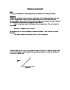
Table 15 shows how the mean resistances change with different lengths of wire. Graph 3 shows a plot of mean resistances against different lengths of nichrome. This showed a good straight line through the origin.
The errors in the measuring apparatus used were:
errors in Ammeter ± 0.01A; errors in Voltmeter ± 0.01V; errors in ruler ± 1mm.
I calculated the percentage error using the formula:
% error = [absolute error ÷ value] x 100
The combined error in Resistance was calculated using: R = (V ÷ I) ± Σ(% errors)
Resistance absolute error was calculated by:
(R % error) x R
100
The error calculations are shown in Tables 7 to 14.
Table 7. Current and Voltage Measurements for 26swg (0.44mm) Nichrome of Length: 80.0 cm, and Error Calculations
Table 8. Current and Voltage Measurements for 26swg (0.44mm) Nichrome of Length: 70.0cm, and Error Calculations
Table 9. Current and Voltage Measurements for 26swg (0.44mm) Nichrome of Length: 60.0cm, and Error Calculations
Table 10. Current and Voltage Measurements for 26swg (0.44mm) Nichrome of Length: 50.0cm, and Error Calculations
Table 11. Current and Voltage Measurements for 26swg (0.44mm) Nichrome of Length: 40.0m, and Error Calculations
Table 12. Current and Voltage Measurements for 26swg (0.44mm) Nichrome of Length: 30.0cm, and Error Calculations
Table 13. Current and Voltage Measurements for 26swg (0.44mm) Nichrome of Length: 20.0cm, and Error Calculations
Table 14. Current and Voltage Measurements for 26swg (0.44mm) Nichrome of Length: 10.0cm, and Error Calculations
Table 15. showing errors in the length of Nichrome 26swg wire and the resistance.
Analysis and Discussion
The purpose of this study was to investigate the relationship between the resistance and the length of nichrome wire. Firstly I demonstrated that nichrome wire, which I selected for this study is a good Ohmic conductor (obeys Ohm’s law). I showed this by plotting graph of voltage against current.
For the investigation I predicted that as the length of the nichrome wire increases, the resistance of the wire increases proportionally. This can be described by the equation:
R ∞ L or R = kL, where L is length, R is resistance and k is a constant.
My results confirm my prediction that as length of the wire increases, so does the resistance (Table 15). Graph 3 shows a plot of Resistance (y-axis) against Length (x-axis). The graph show a good straight line graph through the origin, which means that resistance is directly proportional to the length of the wire. This can be seen from the graph, if the length of the wire is doubled, the resistance of the wire is also doubled. To check how good the linear relationship was between resistance and length from the data in Table 15 and the points in Graph 3, I calculated the product-moment correlation coefficient. I calculated the product-moment correlation coefficient, r, using the equation:
r = Sxy _
√( Sxx Syy)
Table 16. Calculation of Product Moment correlation coefficient (r) for resistance vs. length graph.
Sxx = Σ x2 – (Σ x)2 Sxx = 0.42
n
Syy = Σ y2 – (Σ y)2 Syy = 20.8038
n
Sxy = Σ xy – (Σ x Σ y) Sxy = 2.96
n
r = Sxy _ r = 2.955 _ _ r = 0.999
√( Sxx Syy) √(0.42 x 20.8038)
If the value of r is +1 then the correlation is a perfect positive linear correlation; if r is -1 then the correlation is a perfect negative linear correlation; and if r is 0 then there is no linear correlation (Statistics 1). From my results, I calculated r to be 0.999. This shows that the relationship between resistance and length is an almost perfect straight line.
This result agrees with the model of metal conductors. Metals consist of giant lattice structures. In a metal the outer electrons of the atoms are free to move around (delocalised), forming a lattice consisting of positive ions surrounded by a sea of free electrons. The sea of free electrons form the metallic bonds and are also responsible for conducting electricity and heat (Ramsden, A-Level Chemistry). When no current is flowing, the free electrons move randomly throughout the conductor. Since the electrons move randomly there is no net movement of charge in any direction. When a power supply is connected across the wire, it causes the electrons to move from negative to positive. The electrons then collide with the fixed (vibrating) metal ions. The electrons are continuously gaining energy from the supply and giving it to the ions when they collide and the metal gets hotter. The constant acceleration and collision results in a steady slow drift along the conductor, superimposed on top of the random high velocities (NAS Electricity by Ellse and Honeywill; Physics. by Muncaster). The vibrating ions in the metal lattice obstruct the passage of the electrons. Therefore as the length of the wire increases, the number of obstructions increases proportionally. An increase in the obstructions, increases the resistance.
The resistance of a wire, not only depends on its length but also its thickness and shape (Physics 1). A thick wire has less resistance than a thin one. This is because as the cross sectional area increases, the number of gaps between the obstructing ions increases, and so resistance drops. This can be seen from Graph 2, which shows that the resistance is inversely proportional to the cross sectional area (i.e. the graph is of the form y = a / x , where a is a constant). Resistance also depends on the type of material. The property of the material is called its resistivity. Therefore, resistance can be written as:
Resistance = resistivity x length _
Cross sectional Area
R = ρ x l .
A
Or
Resistivity = Resistance x Area.
Length
In my graph of resistance against length (Graph 3), the gradient represents resistance divided by length. I calculated the gradient to be 6.2Ω ÷ 0.87m = 7.13 Ωm-1. To calculate resistivity of my nichrome I multiplied the gradient by the cross sectional area [π x (2.2 x10⁻⁴)2 = 1.52 x 10⁻⁷m2] which gives a value of ρ = 1.52 x 10-7 x 7.126 = 1.083 x 10⁻⁶ Ωm = 1.1 x 10⁻⁶ Ωm (2s.f.). The value for resistivity ρ of nichrome is 1.08 x 10⁻⁶ Ωm (3s.f.) (Goodfellow). My result is in excellent agreement with this value.
I estimated errors in my resistances and lengths, and the results are shown in Tables 7 to 15. I plotted absolute error bars on my graph of mean resistance against length (Graph 15). I then drew the maximum gradient and the minimum gradient also on the graph (Graph 15). I calculated the maximum gradient as follows:
Gradient = ∆y / ∆x = ∆R / ∆L = (6.8 – 0.6) ÷ (0.88 – 0.1) = 6.2 ÷ 0.78 = 7.948717
= 7.95 (3s.f) Ωm-1. .
I calculated the minimum gradient as follows:
Gradient = ∆y / ∆x = ∆R / ∆L = (5 – 1) ÷ (0.76 – 0.12) = 4 ÷ 0.64 = 6.25 Ωm-1.
To get an estimate of the error on the resistance against length graph, I averaged the difference between the maximum + normal and minimum + normal.
Max – norm = 7.95 – 7.13 = 0.82 and Min – norm = 6.25 – 7.13 = – 0.88
(0.82 + 0.88) ÷ 2 = error in gradient = 0.85.
To convert absolute error into precentage error I used
% error = [absolute error ÷ value] x 100
% error = [0.85 ÷ 7.13] x 100 = 11.9%
To calculate error in resistivity, ρ, I used the formula:
ρ = Gradient x Area = 7.13 x (1.52 x 10-7).
Gradient % error + % radius error + % radius error =
11.9 + 4.5 + 4.5 = 20.9%
ρ = 1.095 x 10⁻⁶ + 20.9%
ρ = 1.095 x 10⁻⁶ + absolute error
ρ = 1.095 + 0.23 x 10⁻⁶ Ωm
Evaluation:
My experiments worked very well. From my preliminary studies, nichrome was the best material to study. This material seems to give more reliable resistance value than any of the other tested metals. Also nichrome showed higher resistance values, whereas for copper resistance was so low that it was difficult to measure.
In my final experiment I obtained a good resistance-length straight line graph passing through the origin. This was confirmed by calculating the product-moment correlation coefficient which gave a value of r = 0.999. This shows that the graph of mean resistance against length is an almost perfect linear relationship (Statistics 1). This makes me confident in my results.
From my graph of resistance against length I calculated resistivity of nichrome to be 1.095 x 10⁻⁶ Ωm = 1.1 x 10⁻⁶ Ωm (2s.f.). The errors in this value was ρ = 1.095 + 0.23 x 10⁻⁶ Ωm. Nichrome is a material consisting of 80% nickel and 20% chromium and a small amount of other elements. The resistivity will change depending on the exact composition. Although I do not know the exact composition of my nichrome ρ result is in excellent agreement with the value of 1.08 x 10⁻⁶ Ωm (2s.f.) for Nichrome V.
My experiments had two types of errors, random and systematic errors (Physics 1). To keep my random errors low I used the same ammeter and voltmeter for the experiments. I also used the same nichrome wire (different nichrome wires may have different composition and slightly different cross sectional areas). Measuring length with a one metre ruler introduced errors but I minimised the errors in diameter measurements using a micrometer. I could reduce random errors by producing many more measurements (e.g. V and I readings). I only recorded 6 measurements for determining the resistance as I did not have time to do more. My biggest errors are probably in the measuring the radius of the wire. I cannot be sure the wire is the same radius all the way along. I only took 2 measurements and should have taken more. My experiments had systematic errors. For example, I had to measure the length of the wire by eye using a 1m rule. However, I do not think my wire was perfectly straight although I tried to keep my eye perpendicular to the rule when recording the length. I could apply tension to the wire to make the length more accurate (straighter). I could improve my Current and Voltage measurements using digital meters reading to 3 decimal places. I read to only to 2 decimal places which results in large errors. I also do not know if my Voltmeter and Ammeter are calibrated properly. Another small error in the determination of resistance of the conductor, which cannot be eliminated, is due to the circuit design used (Fig.2). The voltmeter registers the potential difference across the resistor (conductor), but the ammeter records the current through the resistor “plus” that drawn by the voltmeter. This error will be very small if the resistance of the voltmeter is very high. But this error cannot be removed altogether (see Physics by Muncaster).
Bibliography:
Cambridge Advanced Sciences Physics 1. By David Sang, Keith Gibbs, and Robert Hutchings.
Goodfellow: Nickel/chromium Ni80/Cr20.
NAS Electricity and thermal physics. By Ellse and Honeywill.
Physics. By Roger Muncaster.
Ramsden. Advanced-Level Chemistry, 4th edition.
Statistics 1. By Greg Attwood, Gill Dyer and Gordon Skipworth