We have that n=10 and p= , so
This information tells us that Adam usually wins 7 points, although sometimes he might score a couple of points below or above the mean. It is very unlikely for him to get more than 8 points or less than 4.
Part 2: Non-extended play games.
2. Different ways in which a game might be played.
The first thing we must do if we want to know all the different ways a game can be played is find the domain of Y, the number of points played. Because a player must score at least 4 points and maintain a difference of at least 2 points to win, we can already begin to list the possible values of Y and all the possible score combinations in which a match can end:
Y= 4,5,6,7→
4-0
4-1
4-2
4-3
The combinations are so limited because the game cannot go over 7 points, and if a superiority is not established before 6 points deuce is called. Another observation we must make before writing out the different combinations is that, in order for the game to end, the last point must be scored by the winner. If the last point is not scored by the winning player, then the game goes on until either one wins. For example, if the match is at 3-0, the winner must score the next point or else the game goes to 3-1 and does not end. Again at 3-1, the winner must score the last point or the game goes on.
Given all of this information we can begin to form our combinations. Because the winner has to score the last point, the possible combinations will look like this:. This means that the winner can score 3 out of the 4 points in any order he wants, but he must always score one last. So out of the remaining Y-1 points, he can score 3 in any order. This is a little different for the first combination (4-0), where there is only one possible way of scoring 4 points in a row. Now we can calculate the different ways one player can win:
1+4+10+20
35
Because these are all the ways one player can win we have to double it, which gives us 70.
3. Probability vs. odds that Adam wins.
The model used for this part of the investigation will be the following:
This model only changes when the score ends in 4-0, in which case it would look like this:
The probability that Adam wins can then be found by adding the probabilities that he wins for every different combination.
4-0→
4-1→
4-2→
4-3→
Ben will be exactly the same but switching and around:
4-0→
4-1→
4-2→
4-3→
We can perform a quick check on ourselves by adding both probabilities and finding that they give. Thus, the odds that Adam wins the game are : or 4.77:1. Note that this is not the only way to solve this problem; there are many different approaches. The answer, though, will always be the same.
4. Generalizing the model to fit random probabilities.
If we are going to generalize the model to fit any random probabilities c and d we should first simplify it with summations. The first case is a little different so it will go separately:
Where Y still represents the number of points played.
Because and will always be 1, they can be omitted from the final model. That said, we can write out the model for the probability that Player C wins:
Note: The Combination is represented with a capital C, whilst the variable is a lowercase c.
Part 3: Extended play games.
5. Theoretically endless games.
This point in the investigation gets very tricky, as it becomes very easy to make a carless mistake that can provide us with the wrong numbers. The main difference here with our previous model is that now, whereas before it was. In other words, the total number of points played now does not need to be less than 7. However, because 4 is still the minimum amount of points required to win a match, the cases of still apply as the “non-deuce cases.” With this in mind we can already separate three probabilities which will be unaffected by whether the game goes to deuce or not:
From this point on, if the game goes past 6 points it means that a deuce has been called. However, the game cannot be settled at 7 points because a superiority of 2 points is required. This means that if deuce is called at 6 points, and both Adam and Ben win one point again, deuce will be called once more. If A is a point won by Adam and B a point won by Ben, it would look like this:
AAABBB (+ all other possible combinations for the first deuce) AB
AAABBB (+ all other possible combinations for the first deuce) BA
For the game to end at 8 points the same player must score two points consecutively:
AAABBB (+ all other possible combinations for the first deuce), AA
AAABBB (+ all other possible combinations for the first deuce), BB
This basically states that once the first deuce is called the games can only end on an even number of points. Either way, the probability of the game going to the first deuce should be calculated if we want to know what the probability of the consecutive deuces is. The probability of going to the first deuce, P(d), is a simple binomial distribution:
So the probability of Adam winning or Ben winning after the first deuce is simply:
or
Because every deuce is dependant on its predecessor, we cannot simply find the probability of going to third deuce by increasing the values in the previous model. This means that if we want to find the probability of the third deuce taking place we will have to add the probability of the first, second and third deuces. Therefore, the probability of a deuce taking place is the sum of a geometric series. On top of this lies the fact that the first deuce is different from the rest since it requires 6 points and not just 2. Now we know that the first deuce should be considered separately from the rest of the deuces. Once we have defined this part of the investigation we can find what the probability of any deuce after the first is.
The deuce number that the players are on will thus be represented as. This is so because the point they are on must be subtracted by 8 to find how many points from the first deuce they are (as this includes the two points after the first deuce). Because every deuce is composed of 2 points, multiplying will double Y and hence form a deuce. Now we can find the probability either player has of winning after going to deuce:
Where P can be P(A) or P(B).
However, we must add to this the probabilities that either payer wins without reaching deuce, when Y=4,5,6. So the final model will look like this:
For P(A)→
For P(B)→
For now we will only look into solving for P(A). This will be done through the use of a simple spreadsheet like the following:
The probability of winning is the same as the Sum of the probabilities of winning deuce and non-deuce games. We can find P(B) through the use of a similar spreadsheet but changing the values to fit in for P(B):
Now that we know P(B) and P(A) we can find the odds Adam has of winning against Ben:
P(A):P(B)
0.8530 : 0.1433
5.95: 1.00
This proves that Adam’s game odds are almost 6:1 compared to Ben’s
6. Player C plays extended play games.
The formulas for Players C and D are very simple to write as they are the same as the ones that we used in question 5. The formula for the probability that Player C wins is the following:
With this equation we can form the spreadsheet:
7. Expressions that represent the odds.
The expression that represents the odds is simply. Analyzing the spreadsheet we came up with for question 6 helps us understand what happens when point-winning probabilities are close together or very different. When point-winning probabilities are close together, the odds one player has against the other tend to be closer to 1:1. For example, when P(c) is 0.5, P(d) will also be 0.5, so P(C) and P(D) will inevitably be very similar. The odds I calculated here were simply 0.98:1.00, which means that in this scenario players C and D have a similar level of skill. Other cases, like when P(c)= 0.55 also help to prove this point. However, only a 5% difference can prove to be pretty significant. By looking at how the odds increase with respect to the increase in the point-winning probability we can conclude that there is an exponential relationship. When P(c) increases from 0.6 to 0.7, the odds only increase by about 6:1. In contrast, when P(c) increases from 0.7 to 0.9, the odds increase by over 600:1. The increment in odds clearly does not show a linear relationship with the point-winning probabilities.
If we use our Graphic Display Calculators we can easily obtain the correlation coefficient (r) of the exponential regression for the different odds. The value for the correlation coefficient for an exponential regression is 0.99. This indicates that the relationship is strongly exponential as it has a very strong correlation with all the points. The following is a graph of odds versus point-winning probabilities:
8. Usefulness, limitations and conclusion.
The most obvious limitation to our model is that after all our calculations and finding that Adam’s odds are almost 6:1 against Ben’s, Adam may still loose. I talked about this briefly in my answer to question 1, where the validity of our first model was debated. I find the whole investigation to revolve around one undeniable idea: It is all hypothetical. I reiterate that the accuracy of our models lies only in the meaning of “often enough” (“Two players have played against each other often enough to know that […]”). In the real world, there would be no such thing as “often enough,” since there would always be a margin for error. All this tells us is that when we use our models we must be cautious and always be aware of the fact that they are only predictions. Unfortunately, there is always a small chance that these predictions may be completely wrong. I do not believe that this means the models are useless though, as they can still prove useful for large spans of time. In other words, our models will work better when we deal with averages than when we deal with specific events.
An interesting field of further investigation for this portfolio would be to compare how different distributions can apply to the tennis games. For example, Poisson distribution. In question 1 we found that the expected value for X was about . If we use this as λ we can try to find the probability that Adam scores X number of points in a match. We can use Excel to construct another simple spreadsheet, this time showing the Poisson distribution:
The following spreadsheet is the same, only that it shows the Binomial distribution:
The following is a comparison between both probabilities:
It is interesting to observe that when using different distributions the probability values can vary. Regardless, the correct method is binomial, as a Poisson distribution could technically still work for x=11. What I mean by this is that since the binomial distribution is restricted by the presence of n, it will most likely be more accurate as its values will add up to one. The Poisson distribution, on the other hand, will not always add up to exactly one for the value of n we are using.