SL Type I Mathematics Portfolio

Infinite Summation

Infinite series are among the most powerful and useful tools that you will encounter in calculus. They are among the major tools used in analyzing differential equations, developing methods of numerical analysis, defining new functions, and estimating behaviour of functions, and much more. The use of infinite series can be found in a variety of fields, such as electronics engineering, micro-economics, mathematics, and physics.

In this Mathematical portfolio, the investigation of the sum of infinite sequence, , where: t0 = 1, t1 = , t2 = , t3 =, … , tn =.

For a positive integer, factorial , written as , is the product of all of the positive integers less than or equal to .

Furthermore, (by definition)

This can be proofed with the equation

The above sequence is called an infinite sequence, because the three dots at the end of the sequence indicate that the sequence continues indefinitely. However, the following sequence is called a finite sequence because it has a finite number of terms, . After determine this sequence as an infinite sequence, we should determine whether or not this sequence is convergent or divergent. This is important because if this sequence diverges, the general statement would be . A convergent series is a series in which the terms decrease in magnitude rapidly and for which the sum of the first several terms is not too different from the sum of all of the terms of the series. The following is an example of a divergent series.

Thus, there is no general statement to represent the infinite sum of this sequence. In order to detect whether the given sequence is a convergent sequence or not, there are 3 tests that can prove it. The ratio test is the most comprehensive, and useful test.

Is less than 1, the sequence converges.
Is greater than 1, the sequence diverges
Is equal to 1, the test fails to give conclusive information

We can use the ratio test to determine whether or not our sequence is converging.

Since the 0 is less than 1, the series converges. This determines that the sum of this series is a real number.

To determine the general statement that represents the infinite sum of this general sequence, we must start step by step: (all of the answers below will be corrected to 6 decimal places)

First, we have to calculate the sum of the first terms of the sequence for , for where :

Relation between and (

By using Microsoft Excel, it is possible to graph the relation between and .

This is a preview of the whole essay

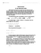
First, we have to calculate the sum of the first terms of the sequence for , for where :

Relation between and (

By using Microsoft Excel, it is possible to graph the relation between and .

I noticed that from this plot, the value is increasing when the value increases, however, the graph does not go beyond . We can say that there is an asymptote at Furthermore, it is noticeable that as , the values of , which in this case is the . Even though on the table, the data shows that when n=10, . This does not mean that the graph is intersecting the asymptote, however, this occurs because we can only take 6 decimal places. When I expand the number, it shows that 1.9999999995. This can be applied to parts of this investigation.

This case can be further proved by inserting

Relation between and (

Again, let’s graph the relation between and .

This plot further proves that the value is increasing while the is also increasing. This time, the graph would not go beyond . We can say that the asymptote of this graph is The observation that I made in the first case can be validated by the fact that as , the values of , in this case it is 3.

Right now, I will calculate the sum , when , and different values of . The 3 different values of is . During this process, it is clear that the cannot be a negative value or zero. This is because to the power of any number will give you a positive number greater than 0. In another word, the domain of is for the positive numbers only. We cannot take the logarithm of a negative number or zero.

Relation between and

From this set of data, I can see that the value is approaching 15, as the value approaches 10. The asymptote in this plot is . The line cannot cross or intersect with .

Relation between and

From this set of data, I can see that instead of increasing exponential until , the relation between Relations between fluctuates up and down, and then it reaches . However, my observation still stands as when as , the values of . In this graph, I noticed something that has not happened with a, the graph fluctuates up and down. I observe that when , the graph dips below the asymptote at . This is due to the fact that , the answer is negative. When the is an even number, the negative values cancel each other out, thus producing a relatively larger number. However, when the is an odd number, the would be relatively low, and often a negative number. Thus, the graph would fall below the asymptote when . The graph will fluctuates above and below the asymptote, but never intersecting the asymptote.

Relation between and

This set of data sees a lot more fluctuation than the last set of data when This is also the first time that is less than 0, when . This is because that the produce a number that is too small. The graph would continue to fluctuate until . Even though this graph has a big fluctuation, it can still take the observation that as , the values of

After investigating the cases above, it is certain that when , the general statement that represents the infinite sum of the general sequence is as , the values of . This can be written as the following:

Right now, we will expand this investigation to determine the sum of the infinite sequence

We can define that as the sum of the first n terms, for various values of .

Let a =2. Calculate for various positive values of .

Using technology, plot the relation between and . Describe the relationship.

Relation between and

From this set of data, I can see that this graph resembles an exponential function : . The function is increasing at an exponential rate. As the x values increases, the values of T9(2,x)would also increase as a result. Thus we can say that . By looking at the graph, we can see this graph takes on the base of 2. This is because in part 1 of this investigation, we have came to realize that as , the values of . This can be written as the following.

This can be further expanded with this investigation.

By sketching the function , I can examine that the function resemble our own plot. Thus, I notice that as the varies, the values of always approach the values of . Further differences will be explained in the next example.

Relation between and

In this example, I can observe that this relationship resembles the function . The only difference between this example and the example above would be the in the function. As I have mentioned above, as the x values increases, the values of T9(3,x) would also increase at an exponential rate. Therefore, based on my observations above, this relation should resemble that of the function. .

After plotting the points for the function , I noticed that most of the points are very similar between both graphs. However, I did remark that when which is not accurate with the function . To enhance that this is not an error, I calculated, that when . The reason behind this will be further discussed in the final conclusion coming up.

General Statement

As the value approaches , the values of will approach This relation can be modeled by the following:

The below domain restrictions can apply to this general statement

is a restriction because we cannot take the common logarithm of a negative number or 0.

. This is because when our sequence looks like this:

When , our sequence is , according to our math textbook, (Patrick 198). . By taking 0 to the power of 0, we will not

As I have mentioned above, even though the value can be very close to , there are other times when the value can be off. As noticed in the example, when which is not accurate with the function . This is because I am only taking the 9th term of this sequence. If I take , the answer would be closer to This pattern can be noted that as the the number of terms that required for would also increase. This can be further mentioned that as the , the number of terms that required for will increase as well.

This general statement is an example of the Maclaurin series. It is a series that expresses a function in terms of an infinite power series whose nth coefficient is the nth derivative of f(x), evaluated at . The Maclaurin series The Maclaurin Series can be written as this :

There are also some common functions of the Maclaurin series. The expansion of by the Maclaurin series is written as followed:

This validates that my general statement - is true.

Here are more values of to test the validity of the general statement.

From the last two tables, we witness that even though the x value is negative, it still does not change the general statement.