Method:
Working out the dilution:
Before starting the experiment a formula had to be used in order to produce a series of dilutions. The series of dilutions included neat (undiluted), 1:2, 1:5, 1:10, 1:20 and 1:100. The formula used to prepare this was the amount required (mls)/dilution factor. So for example to produce the solution 1:2, 5ml of neat food dye and 5ml of distil water would need to be added. So by using this formula:
Amount required (mls)/dilution factor, the values needed for this experiment can be added in as follows:
10mls/2 = 5ml of food dye required to make the solution
Here Table 1 shows the amount of food dye added and the dilution added (in mls) to show how much was needed in order to make up each solution.
Table of Dilution Used:
Table 1
- A sample of coloured liquid was diluted with water to produce a serial dilution series as follows:
- Neat (undiluted)
- 1 in 2
- 1 in 5
- 1 in 10
- 1 in 20
- 1 in 100
- Whilst using conventional and reverse pipetting both 100µl and 200µl samples of each dilution was pipetted into the wells of a 96-well plate.
- Once the pipetting was finished an automatic plate reader was set at a wavelength of 450nm to measure the optical density of each well then the results were printed out.
- The 96-well plate was separated in order to put in the different solutions and measurements. This was first done on paper and this can be seen in appendix A.
Results and Calculations:
Mean of each dilution for the 100µl and 200µl samples:
The mean of each of the four replicates of each of the dilutions for both the 100µl and 200µl will need to be calculated. To calculate the mean the four replicates of the dilutions for both the 100µl and 200µl will need to be added together and then divided by four since there are four samples and thus the mean will be calculated.
So far example to work out the mean of the neat (undiluted) dilution for 100µl, all the four values will have need to be added together. So from looking at appendix B, the values are 2.755, 2.723, 2.743 and 2.698. When added together this would give the sum of 10.919, since there were four values used in this calculation 10.919 will then be divided by four which would give a rounded value of 2.730. So the mean of the neat (undiluted) dilution is 2.730.
Table of Mean Value for the 100µl Sample:
Here Table 2 shows the mean for the 100µl dilution sample.
Table 2
Table of Mean Value for the 100µl Sample (Reverse Pipetting):
Here Table 3 shows the mean for the 100µl sample which involved reverse pipetting.
Table 3
Table of Mean Value for the 200µl Sample:
Here Table 4 shows the mean value for the 200µl sample.
Table 4
Table of Mean Value for the 200µl Sample (Reverse Pipetting):
Here Table 5 shows the mean for the 200µl sample which involved reverse pipetting.
Table 5
Standard Deviation of each dilution for the 100µl and 200µl samples:
After working out the mean, the standard deviation will next need to be worked out for each dilution for both the 100µl and 200µl samples and reversed samples. To calculate the standard devia+tion the mean would need to be subtracted individually from each of the values given. Afterwards this result would then need to be squared and the sum of all the squared values would next need to be done and then divided by n-1 (where n represents the number of values present). Finally this result would then need to be squared rooted and the standard deviation will be found.
For example to work out the standard deviation of the dilution 100µl neat (undiluted) sample, the mean was 2.730 would need to be subtracted individually from each of the values given from appendix B. So 2.730 will need to be subtracted from 2.755, 2.732 and 2.698 which would give the values of -0.025, 0.007, -0.013 and 0.032. These results would then need to be squared giving the results of 0.000625, 0.000049, 0.000169 and 0.001024. The sum of these values comes to 0.00187 which will now be divided by 3 (n-1) which results in 0.000622333. Finally the square root of this would give 0.025 when rounded up. Thus the standard deviation for the dilution (100µl sample) neat (undiluted) is 0.022.
Table of Standard Deviation for the 100µl Sample:
Here Table 6 shows the standard deviation for the 100µl diluted sample.
Table 6
Table of Standard Deviation for the 100µl (Reverse Pipetting) Sample:
Here Table 7 shows the standard deviation for the 100µl (reverse pipetting) sample.
Table 7
Table of Standard Deviation for the 200µl Sample:
Here Table 8 shows the standard deviation for the 200µl sample.
Table 8
Table of Standard Deviation for the 200µl (Reverse Pipetting) Sample:
Here Table 9 shows the standard deviation for the 200µl (reverse pipetting) sample.
Table 9
Discussion:
Explanation of the Raw Data and Results:
Table 2 shows that the neat (undiluted) dilution had the highest mean; also it was the highest for the 100µl reverse pipetting, 200µl sample and the 200µl reverse pipetting. The dilution with the lowest mean result was the 1:100 dilution. This is a positive sign that the reproducibility of the pipetting was accurate since the tables from 2-5 shows that the volumes went from high to low. Thus showing that the more diluted the neat food dye was the higher the mean of the optical density and the less diluted the food dye was the lower the mean of the optical density. This is due to the fact that the more optical dense a solution is, the impact of the wave will be slower. Since the dilution of 1:100 has the lowest optical density this would mean that the wave is able to move past the solution since most of it is just made of distilled water.
For the standard deviation result the 1:100µl dilution had the least value, except in the 100µl sample. This show there may have been an error after all in the pipetting. This may be due to not correctly setting the right measurement, or failing to clean out the plastic tip after using it with the neat food dye then using it with distilled water. This can cause cross-contamination and thus affect the outcome of the results.
Findings of the Graph of Sample Dilution vs. Optical Density:
As we can see from each of the graphs (from appendix C-F), the neat (undiluted) solution had the highest optical density. As the concentration of the food dye dilution decreased so did the optical density. From appendix C which is a graph of simple dilution against optical density (100µl sample) there appears to be an anomaly in the result. This could be due to error of pipetting such as not pipetting the correct amount or not making sure that all the contents from the plastic tip have been pipetted out.
Conclusion:
As we can see from these results the null hypothesis can be rejected since there was a significant difference between pipetted dilution samples and the optical density of each well. As the dilution increased so did the optical density for each of the wells.
The neat (undiluted) food dye solution had the highest optical density because once it was inside the automatic plate reader the waves were moving more slowly through this dilution than the 1:100 food dye dilutions.
References:
Collins, C.H., Falkinham, J.O., Grange, J.M. and Lyne, P. (2004) Microbiological Methods (8th edition) Arnold, London
Daub, G.W. and Seese, W.S. (1996) Basic Chemistry, Prentice Hall, New Jersey
Hoggett, J., Jelrsch, A., Pingoud, C., Urbanke, C. (2002) Biochemical Methods: A Concise Guide for Students and Researchers, Wiley-VCH, Germany
The Physics Classroom, 2011, Optical Density and Light Speed [online]
Available at
[Accessed 13th January 2011]
Appendix: