Yr 9 scatter graph
For this scatter graph I’ve chosen 7 girls and 6 boys making a total of 13 data points. As you can see from the graph above that the data is spread from 1.5m to 1.76m on the x-axis whilst the range for weight goes from 41kg to 72kg on the y-axis. The line of best fit has an equation y=11.38x+42.08. The correlation coefficient for this scatter graph is 0.1141 which shows that there is a strong poor correlation between height and weight thus aiding my hypothesis in me trying to prove that there will be a poorer correlation between height and weight as age increases.
Yr 10 scatter graph
For this scatter graph I’ve chosen 5 girls and 5 boys making a total of 10 data points. As you can see from the graph above that the data is spread from 1.54m to 1.75m on the x-axis whilst the range for weight goes from 42kg to 72kg on the y-axis. The line of best fit has an equation y=41.38x-10.76. The correlation coefficient for this scatter graph is 0.2433 which shows that again there is a strong poor correlation between height and weight thus aiding my hypothesis in me trying to prove that there will be a poorer correlation between height and weight as age increases.
Yr 11 scatter graph
For this scatter graph I’ve chosen 4 girls and 4 boys making a total of 8 data points. As you can see from the graph above that the data is spread from 1.52m to 1.80m on the x-axis whilst the range for weight goes from 42kg to 92kg on the y-axis. The line of best fit has an equation y=25.39x+14.44. The correlation coefficient for this scatter graph is 0.1408, which shows that again there is a strong poor correlation between height and weight. This has proved that my hypothesis is right.
I will now compare the correlation coefficient in a bar chart to make my hypothesis clearer and to prove that it is right. This is shown below.
As you can clearly see from the graph above, the correlation coefficient tends to get poorer as you go up each year; year 7 and 8 have quite a good correlation between height and weight compared to year 9, 10 and 11, whose correlation is pretty poor. This proves that the first part of my hypothesis is correct.
I am now going to show that the last part of my first hypothesis is correct-boys will tend to have better and stronger positive correlation than girls in each year group. To do this I am going to draw up several scatter graphs for boys and girls in each year group and compare them. I am also going to compare the correlation coefficient of boys and girls in each year group, similar to what I did earlier.
Scatter graph for year 7 boys
Correlation coefficient for boys in year 7- 0.4594
Scatter graph for year 7 girls
Correlation coefficient for girls in year 7- 0.4001
As you can see from the two graphs above, I have so far proved my hypothesis right and this is backed up by the correlation coefficient which is stronger in boys than girls (0.4594 and 0.4001 respectively)
Scatter graph for year 8 boys
Correlation coefficient for boys in year 8- 0.3526
Scatter graph for girls in year 8
Correlation coefficient for girls in year 8- 0.5454
Scatter graph for boys in year 9
Correlation coefficient for boys in year 9- -0.1243
Scatter graph for girls in year 9
Correlation coefficient for girls in year 9- 0.2861
Scatter graph for boys in year 10
Correlation coefficient for boys in year 10- -0.7942
Scatter graph for girls in year 10
Correlation coefficient for girls in year 10- 0.4528
Scatter graph for boys in year 11
Correlation coefficient for boys in year 11- -0.1609
Scatter graph for girls in year 11
Correlation coefficient for girls in year 11- 0.3508
Table to compare the correlation coefficients of all the year groups and gender.
As you can tell from the graphs above, the third part of my first hypothesis (stating that girls will have a stronger positive correlation than boys) has been proved slightly wrong although it has not been proved entirely wrong and there is some evidence to support my hypothesis.
If you were to look at my first hypothesis you can compare the correlation coefficient of the two (boys and girls) and in the first case boys have a stronger positive correlation than girls (0.4594 to 0.4001). Reasons for this may be found in the conclusion. Year 8 completely support my hypothesis as the girls in year 8 have a stronger positive correlation than the boys in year 8 (0.5454 for girls compared to the boys correlation coefficient of boys being 0.3526). Looking at the graphs for the boys and girls in year 9, my hypothesis has sort of been proved right as firstly you can just tell from the shape of the graphs: girls have a positive line of best fit while the boys have a negative line of best fit. For complete assurance I compared the correlation coefficient of the boys and girls in year 9 and inevitably the girls had a stronger positive correlation than boys (0.2861 for girls and -0.1243 to be precise). It is a similar case for year 10 and 11. looking at year ten, again by just looking at the graphs of boys and girls you can immediately tell that girls have a stronger positive relationship than boys as the boys graph have a negative gradient compared to the girls positive shaped graph and gradient. Comparing the correlation coefficient of the two girls have a pretty decent 0.4528 compared to the boys -0.7942. Similarly in year 11 the correlation coefficient for girls is 0.3508 compared to the boys’ -0.1609. However this part of the hypothesis is slightly wrong as I mentioned that girls will have a stronger POSITIVE correlation than boys. Although not mentioned it was taken that I meant that boys will have a weaker correlation than girls although not a negative one. Reasons for this maybe found in my conclusion.
Conclusion
Overall I reckon that I have made an accurate an educated judgement when stating my hypothesis as you can see above, most of it has been proven correct. Firstly the first part of my hypothesis (there will be a positive correlation of height against weight in the whole school) has been proven correct. This is because height increases with weight almost proportionally for a lot of people and so proving my hypothesis right. Looking at the second part of my hypothesis (there will be a positive correlation between height and weight in all year groups though the correlation tends to be poorer as pupils get older i.e. as you go up the year group). This is because at nearly one
quarter of final adult height results from the teenage height spurt. This happens at the age of between 11 and 13 so assuming most of the pupils within that age group would be in years 7 and 8. While they are growing at such a rate it is at this stage where they balance out their weight: eating a lot of food that nutritious and healthy, needed to maintain a pretty steady growth thus as they grow in height their weight increases proportionally. However in year 9 pupils, according to Dr Bryan Lask from St George's Hospital Medical School, tend to grow less as 75% of their total height has been attained at the age of 11 and 12. Therefore as they have stopped growing pupils are therefore required to maintain their body health including their weight. However researchers have suggested that children around the age of 14 (year 9) go through a phase faced by teenagers where they become lazy and easily “bored” and agitated and therefore eat a lot more to keep them calm apparently and so causing an increase in their weight. Research has also shown that all the laziness has seen teenagers forcing themselves to sleep thus altering their sleep patterns and body processes that happen by a natural process and this apparently leads to an increase in weight. This means that pupils of this age are not growing and are putting on extra weight which means that there will be a poor correlation between height and weight. Similarly for pupils in year 10 and 11; they tend to be more careless and their lack of responsibility and morals leads to them drinking, smoking, sitting in front of the television digging into their high cholesterol food and just taking everything lightly. Research from the American institute of health has shown that children of ages between 16-18 spend a lot more time watching television and spending more hours sleeping and a lot less time engaging in physical activity. This in conclusion leads to a poor correlation between height and weight as pupils in the upper years aren’t increasing in height yet are having a significant increase in their weight.
The third part of my first hypothesis has been proven slightly wrong. For instance the evidence collected for year 7 contradicted my hypothesis (that girls will have a stronger positive correlation than boys). This maybe because at the tender of age of pupils in year 7 boys experience their growth spurts earlier than girls (proven by scientific research). Also boys in year 7 begin to take interest in building their muscles and participate in a lot of physical activity as well as watching their diet. This has meant that they tend to have a very strong positive correlation between height and weight. Girls on the other hand, although experiencing a growth spurt at roughly around the same age it is more significant when they are slightly older (when they are in year 8 or 9). Girls at this age are not thought to engage in a lot of physical activity as boys though are aware and conscience of their weight so there tends to be a pretty good relationship between height and weight but not as good as boys. In year 8 (as mentioned earlier) girls experience a growth spurt which sees them gain 75% of their adult height. At this stage girls are still conscience or their weight and the pressure of looking glamorous at such an early age has seen them once again watching their weight, thus going on things like diets and therefore there is a good relationship between height and weight. For boys, they tend to grow less and become more careless and have no desire to care if their laziness gets the better of them and this could lead to them having an increase in weight so showing a poor correlation between height and weight and although there are more reasons and suggestions as to why there could be a poor or negative correlation with boys, this was my suggestion as I did some background research on teenagers and carefully noted down what it had to say. For year 10 and 11 the cases are very similar to year 9 (same reasons).
MY SECOND HYPOTHESIS
In this hypothesis I will be investigating that if boys have a larger average weight than girls. I will calculate the mode, median and mean for boys and girls grouped and ungrouped data. If the mode, median and mean are larger for boys than girls then this obviously proves that my hypothesis is correct.
Mode- the mode of a set of values is that which occurs the most frequent.
Median- is the middle value when the data is arranged in ascending/descending order. If there are two values in the middle then the average of the two values is taken.
Mean- is the value when all the data points are added up and divided by the number of data points.
I will use autograph to draw my cumulative frequency graphs and calculate the mode, median and mean, though this can be done manually.
Boy’s weight
Ungrouped data for boys
Mean: 54.2
Median: 55.5
Mode: 35,45, 63
Girls’ weight
Ungrouped data for girls
Mean: 52.73
Median: 48
Mode: 45, 48
(Ungrouped)
As part of my investigation I have proved my hypothesis right as you can see from the evidence that I have collected above. I calculated the mean and median using a program called autograph as well as calculated it manually to double check that I’ve done everything correctly. As you can see boys have a larger mean than girls, which means that boys are generally heavier than girls thus proving my hypothesis right. Again, boys have a larger median than girls which seems to suggest that boys have a larger average value than girls so proving my hypothesis right in saying boys have a larger average weight than girls. Boys have the highest mode so it seems to suggest that boys are generally heavier than girls, proving my hypothesis right.
I could also just “shoot up” a stem and leaf diagram just to show that boys have more values in the higher regions of weight (i.e. within 50kg and 70kg) than girls whose values tend to be more concentrated around the lower weights (i.e. with 35 and 60 kg)
STEM AND LEAF DIAGRAM
As you can see from the comparison of the boys and girls in the stem and leaf diagram above you can immediately spot that the girls weight are mostly found on the “40s” region where as boys weight although found in the same region as well more values are found in the higher regions (60s and 70s) than girls thus showing us that boys have a larger average weight than girls. Though this method is not the most accurate ways of carrying out my hypothesis it is a useful measure and helps us to make a rough estimation.
If data was of the whole school was based around this group of 60 pupils I could predict that a girl chosen at random would have a probability of 0.53 to weight between 30/40 kg and a probability of 0.40 to weight between 50/60kg and a probability of 0.06 to weight in the higher region (i.e. around 90/100 kg).
If I was to pick a random boy I could predict that he’s probability of weighing between 30/40kg would be 0.43 and the probability of him weighing between 50/60kg would be 0.53, 0.13 (or 13%) more than the probability of a random girl having that probability. The boy’s chance of weighing between 90/100kg would be 3% or a probability of 0.03, purely based on statistics. So as you can see a boy has a higher chance of weighing more than a girl.
Grouped data for girls
Cumulative frequency graph for girls
Grouped data for boys
Cumulative frequency graph for boys
Comparing the cumulative frequency of boys and girls
Key
Lower quartile mark
Median mark
Upper quartile mark
(Grouped)
As you can see, I’ve grouped all the data. This has yet again proved my hypothesis right, as shown by the cumulative frequency graph above and the results (mean, median) obtained from it; although the mode for both boys and girls lie on the same range you can see that boys have got a higher value for the mean and median proving that boys have a larger average weight than girls and so proving my hypothesis right. The cumulative frequency graphs basically show me what I have calculated in the table above. I have just included it as a sort of assurance to back up my hypothesis for example if you look at the cumulative frequency graph for girls you can notice that it has a very steep gradient in around the median (50%) so seeming to suggest that most of the girls weights are concentrated between 40-50kg and as you can see from the table above, that was what we calculated as the modal group.
If I was to look at the cumulative frequency graphs I worked (using autograph) that the girls have a lower quartile of 45 while boys have a lower quartile of 44.25. On the other hand boys have a higher median and upper value (median for boys’ ungrouped data=55.5 while girls median=48. Upper quartile for boys=63 while girls’ upper quartile=59.25). All this suggests the boys have less values concentrated in the low regions of the weight scale and as you can see (from the median and upper quartile) boys’ probably have more values, than girls, concentrated in the higher regions of the weight scale meaning that the have a larger average weight than girls, proving my hypothesis right.
GREEN FILLED HISTOGRAM- BOYS’ HISTOGRAM
NON FILLED HISTOGRAM-GIRLS’ HISTOGRAM
I have drawn up a histogram, using ‘Autograph’, for both boys and girls and they are being compared on the same statistics page. Firstly you can notice both histograms have a normal distribution. As you can tell girls and boys have the same modal class (group with most set of values), 40-50. However as you can see that boys have less values than girls in the modal class and this is shown by the shorter bar, seeming to suggest that most of the boys values for weight are found in the higher regions and this is proved right by looking at the histograms. As you can see as group size increases boys have more values concentrated in those regions than girls, and this is shown by the taller bars. This seems to say that boys have more values in the higher region so seeming to suggest that they have a larger average weight than girls, proving my hypothesis right.
Conclusion
In conclusion I have proved my hypothesis in saying that boys have a larger average weight than girls. I have proved this in both sets of data I have taken, grouped and ungrouped. Although I have proved my hypothesis right there is not much difference in the average boys’ weight with the average girls weight though boys do tend to have a larger average weight. There are several reasons why this is true. Firstly adolescent girls are thought to suffer from a disease known as coeliac disease which is a disease where the body is gluten intolerant so sees them losing a lot of weight or the inability to gain weight. People suffering from this disease may eat a lot but not put on any weight. This could lead to a disease similar to Osteoporosis (osteoporosis is suffered by older women), which is a disorder where the bones become weakened by loss of substance and results in bone mass reducing by 1% every year. This disease (coeliac) is more significant in girls and the disease similar to osteoporosis see’s girls losing their bone mass at a faster rate than girls.
Hormones, such as estrogen and cause an increase in weight in both girls and boys. The skeleton in girls grows much the same way as in boys however boys end up having a structure where the bones are much heavier and denser thus meaning that boys will tend to be heavier than girls.
Another proposed reason as to why boys have a larger average weight than girls is the fact that girls (and boys to a lesser extent) are affected by the ‘slimmers disease’-anorexia nervosa. Research shows that boys are 4 times less likely to suffer from the disease than girls. Symptoms include; loss of weight, refusal to eat, abnormal fear of being fat and a desire to be thin. All this leads to having a slimmer body and being thinner and less heavy than boys. Also teenage girls are far more likely to diet than boys (even if they are not overweight) and this is due to the growing pressure of looking glamorous which is not that significant in boys. Researchers have shown that students of 15 years old 26% of girls are on diets compared to just 5% of boys. Also by 15, 25% of medium weight and 8% of low weight girls said they were dieting compared with under 3% of medium to low weight boys (according to Dr Helen Sweeting, a researcher at the medical research council social and health sciences unit at the University of Glasgow). Recent reports have also shown that Women pregnant with boys tend to eat about 10 percent more calories a day than those carrying girls but don't gain more weight. The study, published Medical Journal, appears to explain — at least in part — why newborn boys are heavier than girls. This would also if mean that the boy would be more likely to be heavier than the girl when they reach adolescence.
Disregarding all the research, from general knowledge I know that boys will tend to be heavier than girls as boys’ bodies are well built and an Increase in muscle strength occurs after an increase in mass. Boys’ muscles begin to come up between the age of 12-18 and as I mentioned earlier, this only occurs after an increase in mass. Girls tend not to experience this so their physique remains pretty much the same and so their weight does not go up as significantly as boys would.
The graphs above are to show roughly how much a girl/boy should weigh between the ages of 1-18. If you were to look and compare the percentiles you can see that at each of them boys will tend to expect to weight more than girls for e.g. at the 75th percentile girls should expect to weigh 68kg while boys are expected to weigh roughly around 79kg. Even at the boys’ 50th percentile it is higher than the girls’ 75th percentile (75kg to girls’ 68kg).
In conclusion my hypothesis in saying that the average boys weight is larger than the average girls weight is proven correct.
HYPOTHESIS 3
My third hypothesis states that people who walk will tend to have a lower body mass index than people who take any other forms of transport. I also stated that people that walk are more likely to fit into their BMI category (i.e. between 20-25).
BMI-Body mass index, or BMI, is a new term to most people. However, it is the measurement of choice for many physicians and researchers studying obesity. BMI uses a mathematical formula that takes into account both a person's height and weight. BMI equals a person's weight in kilograms divided by height in meters squared. (BMI=kg/m2). The chart below shows what the body mass index of people and it tells us of their status.
The final part of my hypothesis states that people who cycle are the one’s who will have the lowest body mass indices compared to the rest of the group (i.e. the people who walk, take the bus or travel by tram).
I can draw up several bar graphs to show prove my hypothesis correct. I can also work out the mean value of all of the values of each different form of transport that people travel by and use the standard deviation to prove a certain part of my hypothesis correct. I can also use a pie chart to show the proportion of people the lie with the “normal” range of BMI and show that the majority of those people walk.
Copy of the data I will use in this hypothesis
Firstly I’m going to draw up a bar chart of average body mass index, which I calculated for each of the different modes of transport taken by people. The bar chart is shown below.
As you can already see my hypothesis has been proven correct twice. The average body mass index of people that walk is well within the range of having a normal BMI. You can also see that people who cycle have the lowest BMI, proving my hypothesis correct. To give accurate numerical values for the values I calculated that helped me draw the bar chart, I’ve drawn to a table below to show the values.
Next, I’m going to draw up a bar chart which shows the percentage of people, in each mode of transport, that have the required BMI for normal weight status. I will do this by looking at the number of people in each “transport category” and then take the number of people the have a BMI of between 19.9-24.9. I will then divide those number of people by the total in that transport category and multiply that value by 100 to calculate the percentage.
As you can see from the graph above (and values that were used to draw up the graph) my hypothesis has been proven correct. As I stated earlier in my hypothesis, that people that walk will have more people that have the required BMI. My graph shows that people that walk have the highest percentage of people of their group (53%) that have the required BMI (compared to the other groups), thus proving my hypothesis correct. In my hypothesis I also stated that people who cycle will have a lower body mass index (or will be underweight) than people that take any other forms of transport. In the results table you can see that they (cyclists) have quite a high proportion, compared to people that take the tram, which have the required BMI(33.33% of cyclists have required BMI compared to just 8.33% of people that take the tram). Does that seem to suggest that people who take the tram are more likely to have most of the people in their category with low BMI hence they will tend to have the highest proportion with the lowest BMI and therefore being underweight and proving my hypothesis wrong (as I stated that people who cycle will have the highest proportion In that region)? No, not necessarily, and that’s why I have made a several other calculations to draw up another bar chart that shows the percentage of people in each group who’s status is underweight (I.e. having less than 19.8 for their BMI).
From the graph above you can see that my hypothesis has been proven wrong. This is because from the graph above I have calculated that people that take the tram have the highest percentage of people (83.33%) that are In the “underweight” category (i.e. having a BMI of less than 19.8) and this contradicts the part of my hypothesis that stated that people who use bicycles as their mode of transport will have the most number of people or highest proportion of people with the lowest BMI (or will be in the underweight category).
HYPOTHESIS 4
For my forth hypothesis I will investigate whether boys have a larger spread of height than girls. To do this I will use several measures to prove my hypothesis right including: standard deviation which shows how widely spread the values are from the mean so if the value for the standard deviation is high that means that the values are spread out. I can also work out the mean, median, lower quartile, upper quartile, lowest value, highest value, range, interquartile range, semi interquartile range. The range is the simplest measure of spread and so it will be quite useful to include it. I will also include variance as it is a natural measure of spread and is provided by the sum of the squares of the deviations from the mean (as I’m using autograph it will work the average of the all the deviations of each point and all I need to do is square it). The more the variation the larger the value and so the more spread out the data is. All this will help me prove my hypothesis as it will give a good comparison of girls and boys and how spread the values are: for example if the lower quartile for a group of values is quite low and the same set of data has a high value for the upper quartile that would mean that it would have a large interquartile range and so proving my hypothesis right. I will also use box and whisker diagrams to explain my hypothesis. In box and skew diagrams a population that is not symmetric (mean and median have similar values) is said to be skewed. A distribution with a long ‘tail’ of high values is said to be positive skewed, in which case the mean is usually greater than the mode or the median. If there is a long tail of low values then the mean is likely to be the lowest of the three location measures and the distribution is said to be negatively skewed. I can use this to show the spread as if the box and whisker showed the data was symmetric that would mean that the mean value will be similar to its median value. This would that these values will be close to that of the mode of the data. This would mean that the data is evenly spread out on both sides of the mean, median and mode thus proving my hypothesis wrong. As you can see I can use the box and whisker diagrams to explain a lot of things on my hypothesis.
I will measure the skew of the data using the formula:
3(mean-median)
Standard deviation
This will help identify the skewness (positive, negative or symmetric).
A rough diagram of a box and whisker would look something like the one below
A positive skew can me noted by
Median- lower quartile < upper quartile- median
A negative skew can be identified by
Median- lower quartile > upper quartile- median
Symmetry is when the distance between the median and lower quartile is equal to the upper quartile minus the median.
I will now use (as mentioned earlier) the program autograph to draw up my graphs (cumulative frequency graphs and box and whisker diagrams) and also calculate values such as the lower quartile, upper quartile etc.
Grouped data for girls
Grouped data for boys
Cumulative frequency graphs and box and whisker diagrams for girls and boys being compared
From the table above I will firstly compare the standard deviation. You can see that for the ungrouped data boys have larger standard deviation than girls, telling us that the data for boys is more spread out from the mean than girls. Boys have a standard deviation of 0.0979484, which is 0.0267328 more than the girls deviation (0.0712156). By doing this my hypothesis has been proven correct. It is a very similar case for the grouped data as well. Boys have a larger spread than girls (0.100571, which is 0.0136483 more than the girls’ deviation of 0.0869227).
Comparing the variance it is inevitable, after looking at the standard deviation, that the variance will show that boys’ weight is more spread as variance is simply “standard deviation²”. Boys therefore have a variance of 0.009593889 which predictably is more than the girls variance (0.005071661) thus proving my hypothesis right once again.
Another measure I can use is the range (highest value minus lowest value), this is because if a range is bigger than another range when comparing data then this shows that the values are spread out because the range is bigger showing that the lowest value is quite low and the highest value is quite high so the values are spread out more as there is a bigger range to be spread around in. the largest value for boys height is 1.8m and their lowest value is 1.36m giving a range of 0.44. Girls’ on the other hand have a range of 0.33 thus showing that boys height is more spread out than girls, proving my hypothesis right. You can also see by the whiskers on the box and whisker diagram (on the previous page) that girls and boys have the same “highest value” but if you look at the lowest value it is more spread than the girls
As I mentioned earlier, we can use the interquartile range to show the spread. The gradient on both the cumulative frequency is quite steep meaning that there will be a small interquartile range. Boys’ ungrouped data have a lower quartile of 1.56 which is higher than girls’ by 0.01 which is not a very big difference. However the boys’ upper quartile (for ungrouped data) is 1.68 which is 0.0375 higher than the girls ungrouped upper quartile of 1.6452 meaning that boys will have a higher interquartile range than girls (as they have a value for lower quartile that is slightly more than the girls lower quartile but at the same time boys have a higher value of the upper quartile than girls). The interquartile range for boys ungrouped data works out to 0.12 (upper quartile-lower quartile, 1.68-1.56=0.12) which is 0.275 more than the interquartile range for girls ungrouped data which works out to 0.0925. As boys have a larger inter quartile range (IQR) it means that boys’ weight is more spread out than girls, proving my hypothesis right once again. However if I was to look at the interquartile range for grouped data, it slightly contradicts what I found by looking at the interquartile range for ungrouped data. For grouped data boys have a lower quartile of 1.55278 and an upper quartile of 1.68036 giving an IQR of 0.12758. On the other hand girls’ (grouped data) have a lower quartile of 1.54643 and an upper quartile of 1.675 giving an IQR of 0.1286714 meaning that girls have an IQR that is 0.0010914 marginally larger than the boys, proving my hypothesis wrong. As the semi-interquartile range is basically half the value of the interquartile range it will inevitably give me the same results (in terms of proving my hypothesis right or wrong) so I found no reason to include it as it will inevitably (after looking at the interquartile range for ungrouped and grouped data) prove my hypothesis right for the ungrouped and wrong for the grouped data as we calculated boys to have a lower IQR in the ungrouped data, proving my hypothesis right where as we calculated boys to have a higher IQR than girls in the grouped data.
Going back to my box and whisker diagrams I calculated girls to have a positive skew while boys’ have a negative skew meaning that the mean is most likely to be less than the mode because of extreme values at the negative end of the distribution. For boys’ ungrouped data, I calculated their skewness as -0.51058 (using the formula I stated in the introduction of this hypothesis. For girls I calculated their skewness as 0.421256 meaning that for both groups (girls and boys) the data is spread. Girls’ data is spread towards the positive end of the distribution (i.e. towards the higher height values near the upper quartile) while boys’ data is more likely to be concentrated towards the negative end of the skew (near the lower quartile). Although one is positively skewed and the other negative I can still compare and comment on the spread using the two values I calculated. I can say that boys’ values are more spread than girls (disregarding whether it is positively or negatively skewed) as the value calculated for skewness for boys is higher than the girls as the higher the value for skewness the more spread they are from the mode of the population. Their graphs for their skewness would look roughly like the ones below. (Positive for the girls and negative for the boys).
However after calculating the skewness for grouped data for boys and girls it sort of contradicts what I concluded from my ungrouped data. I calculated the skewness as 0.5733 for girls while boys’ have s skewness of -0.40896, meaning that the values for girls are more spread, proving my hypothesis wrong.
Another thing I noticed, or worked out rather was that 20% of boys lie below their lower quartile while 16.67% or girls lie below that same value meaning that boys data is more spread than girls below the lower quartile, proving my hypothesis right to an extent. It is a similar case when comparing the percentage of pupils above the upper quartile. Girls’ have 16.67% that lie above their upper quartile while boys have 50% which lie above the same value. This means that because they have a higher percentage it means that they could have a range of heights which means that the data could easily be spread out. To make it unbiased I also compared the percentage of girls above the boys’ upper quartile value, which still worked out to the same value of 16.67% while boys still had a higher value, of 20%, above their own upper quartile meaning that the data was more spread above the upper quartile for boys than it was for girls, proving my hypothesis right. Similar results were obtained for the grouped data so I felt no need to include it as the ungrouped data (for calculating percentages above lower and upper quartiles) already proved my hypothesis right and I would just be proving the same thing again (by using grouped data) using similar methods and obtaining similar results.
Overall I think my hypothesis has gone to plan and been successful in being proven right with the odd contradictions overshadowed by the numerous results that proved my hypothesis right.