Obtaining data
To collect my data I created a spreadsheet in Microsoft Excel and proceeded to enter the titles of data which I needed. These titles included the person gender, their initial estimate of the line, the cm from the exact length after the first estimate, their second length estimate after being shown a different exact length and the difference from the exact length again.
What I did was go round to various people and collected the data for the columns sex, initial estimate of the line and length estimate after being shown a different exact length .The sampling method I used was random, so as to receive a varied range of results, I did not choose just school pupils but adults from out of school so as to make the results varied. From those results I entered them into the spreadsheet I had created in Excel and used a formulae to fill in the columns cm from the exact length after the first estimate and difference from the exact length the second time. The formulae was =9.5-(estimate). This left me with the exact distance from the exact length of 9.5cm. Both the lengths which I showed the people were horizontal way up so as not to confuse anyone. People estimate lengths differently if they see it a different way up. This way the margin or error was decreased. I had collected 50 data entries , and using the formulae continued to work out the distance from the exact length.. This is because the distance is easier to work from in some circumstances such as the averages, but on the whole they basically mean the same thing. From this data I have created and analysed various statistical graphs and charts and entered my findings below.
Table of results
First, below you can see table which I created with all the results entered into them.
As you can see I have sorted them using the sort function in Excel.
Now what I have done is produce 5 graphs . 2 cumulative frequency graphs using the estimated lengths of both attempts, not the differences (see graphs 1.1 and 1. 2). 2 Histogram graphs have also been produced, I intend to analyse the spread on these graphs (se graphs 2.1 and 2.2). A scatter graph has also been created, showing the first estimation differences along the x axis by the second estimation differences along the y axis. IN the next section I will compare the graphs to each other and then conclude on my findings from each graph. From the scatter graph I intend to analyse it and try to find a line of best fit and a gradient. Last of all I intend to analyse the averages which I have found for the differences and the standard deviation.
Analysis and comparison
The cumulative frequency graphs:
As you know, cumulative frequency graphs always go from down to up diagonally, this is because you are adding the frequencies up, it must go up because you are adding frequencies each time, it can never go down. A cumulative frequency graph is used to show the median, the middle point in the data, it also shows how spread out data is. The shape of a cumulative frequency curve tells us how spread out the data values are. A widely spread line (like figure 1.1) means that the data is widely spread out around the median, therefore there is a larger interquartile range. If the line is tight and goes up quicker (between shorter amounts of data), then that means that the data is tightly distributed around median leading to a smaller interquartile range. (like figure 1.2)
You can see that figure 1.1 has a wide cumulative frequency curve, as you can see on the graph, the interquartile range is a lot wider than figure 1.2’s. This would mean to me that after the second estimation, the results show that more people did estimate closer to the exact length after being shown the exact length than during the first estimation. This would mean that the results were very consistent. This information can be defined can shape significance.
So from this cumulative frequency graph, you can see that the results were more tightly packed around the median during the person second estimation. The quartiles, do not show a lot of change except for a 0.1cm decrease for the median meaning the median results was 0.5cm lower than the exact length, and the first estimates median was 0.4cm lower than the median, meaning that , in the case of the median results , the first estimation was nearer. The only other quartile change was the 3rd quartile, the distance was greatly reduced for the second estimate, so this totally contradicts and confuses my results . I will have to analyse more results to find a definite answer.
The Histograms
The histograms show a definite pattern. The use of histograms is to be able to analyse the spread of the data, like a cumulative frequency graph, but better, in that it is in a frequency style. From the mean of 9.5cm , you can see that on figure 2.1, the results are spread quite evenly on both sides, between 9.5cm , the frequencies are exactly the same. Both with the frequencies 11.
The significance of the shapes on a histogram are highly important in that the first results 2.1,show a medium dispersion, the results are kind of equal along the way, leading a “lazy” pyramid shape. This would mean that the distribution is covers a very wide range with many people choosing different results for each column. The second graph shows a much tighter distribution. This time the results are much tighter together, they are within a narrower range and so this lead to a more definite pyramid shape. This leads to a more definite variation for the first estimation graph (figure 2.1) , with the results covering a wider range. The second estimation results show that the frequency results are much tighter together leading to little variation in results for the estimation.
For me this would mean that for the first results, there was a much wider spread of results, there was quite a lot of variation in results and it showed on the graph with high dispersion on the graph. However, on the second graph, the spread or distribution of the results was much tighter, there was a sharp decrease in all the results except for the middle three which all grew. This means that the for the second estimation attempt, people did estimate closer to the exact length of 9.5cm. With the increase in the frequency bars around the median, the sudden and quite large decreases in the surrounding bars, that the spread decreased and was heavily accented around the median areas. The variation in results was now very little and could be seen quite easily. This means that after seeing the exact length , the results became more accurate , as in they were nearer the exact length.
The scatter graph
The scatter graph shows how closely two sets of data are related. It shows the correlation between the first estimation and the second estimation. If the correlation is good, it means the results are strongly related to each other, a poor correlation means that the relationship between the two sets of results is very little. The scatter graph I have produced shows that the correlation between results was quite good. The scatter graph shows a mixed correlation but you can just make out the distinct shape of positive correlation. This would mean that the results are quite closely intertwined with each other and do somehow relate to each other.
If you view all the results the x axis way, you can see that they spread out quite out a bit, from about -3.5cm to 4.0cm. This shows that the spread of the data for the first correlation was quite wide and varied quite a bit. However, when you view the second data results , along the y axis, you can plainly see that these results are much closer together and do not vary as much. From around -2.5cm to about 1.5cm.
I can conclude from these scatter graph results that, like the other conclusions to the other graphs I have analysed, the second estimate results were more accurate.
The averages
From each average I can find out more information about if my hypothesis can be correct or not. I am using the averages I calculated using Excel for the differences. These include the mode, the median, the mean and the range.
Fir the mean, the mean for the first estimate difference was -0.094 and the second estimate difference mean was -0.444. This now leads to a problem, this totally changes everything as so far all my results have led to the second estimate being close to the exact length. However, this mean of the differences clearly shows that the average length of the first estimate from the exact length was nearer to it than the second estimate difference average.
This could be an anomaly within the results which seriously takes down the average , or it could actually be the average. However I seriously doubt this as the rest of the results so far show that second attempt estimates were a lot closer to the exact length, so how can the average distance from the exact length be lower the second time round if all the other graphs say otherwise. I will have to analyse the rest of the averages to reach a conclusion.
The median
I have already discussed the median and what it shows, like the mean, the results show that the middle results was nearer to the exact length the first time round estimating than the second time round after being shown an exact length. Like the mean, this could also mean that an anomaly is somewhere within the second estimate results.
The range
The range is a the pattern of the second estimate results being closer to the average than the first estimate results. The maximum data minus the minimum data for both length differences equals the range. As the range for the second estimation was lower, it would mean that the max or/or minimum decreased by about 2.5 total. Meaning peoples estimation decreased leading to their estimation becoming more exact and my hypothesis being true.
The mode
The mode didn’t really account for much as it was the same for both graphs, this however does not affect my final results one bit, as the mode means the most, and it means peoples estimations were around that area still and did not waver much. However it would have been better if it had been maybe a bit lower as that would have meant peoples estimates changed to be even more exact and I was collected more accurate results than the first estimate.
The standard deviation
The standard deviation is a measure of how far from the mean the data is spread. It is the average distance of data from the mean average. This is very important as it can show if the data has changed to become more accurate, basically a more accurate version of the mode and a histogram mixed together, but much more accurate. The first estimate difference results average came up with 1.936482188 , this was not surprising, as you can see on the histogram the results varied quite a bit. However for the second estimate difference results , the standard deviation was 0.964716306, a large drop and meaning something very important. My hypothesis was correct This large drop mans that average distance from the mean data was decreased meaning the results became closer together and there was less variety and variables between them.
Conclusion:
In conclusion to this, I believe that after careful examination of all the evidence I have collected and the production and comparison of various statistical graphs , I can now say that I believe that my hypothesis was correct. I do believe that peoples estimation of a lines does become more accurate after being shown an accurate length. There is overwhelming
evidence suggesting this information is correct and I do not believe that all this information can be false. In conclusion , I think that many reasons could have affected these results ,but they would not have affected them significantly enough to change them and make the end very different. I will discuss what factors could affect it in the evaluation.
Evaluation
I think that I have analysed and gone through this coursework quite well, I analysed each sector of my hypothesis correctly and did not miss anything important out which could have affected my results. My data collection went fine and I had not problem collecting data as I had already done some a lot earlier when we were first told we had a maths coursework on estimating lengths. At that time I had already devised what I was going to do and set out collecting some data. I only needed a few more pieces to complete the data up to 50. I had no trouble creating and analysing the data and I looked up on the internet about certain statistical information which benefited me a lot, such as the standard deviation. My conclusion was quite hard to write as I had already gone over everything I needed to go over during my analysis so I just concluded on my project.
I don’t think I could make any change to my project, though I could expand upon it in many ways. First I would expand upon the number I data I collect, instead of 50 maybe 100, or 200. Then I could see if the data would reap the same kind of results. I could change the exact length shown and see if that affect the estimation, instead of 110mm, maybe a shorter length like 50mm. Changing the length they have to estimate could also change the results, as in their estimation may be better if it’s a length they could remember well like 15 centimetres. These changes I believe would seriously affect the results I receive and have to analyse. Since I collected the sex of the people in question, I could see if sex affects the line estimation, when analysing the results, I already noted that, either women estimated quite near the lines length or exactly the length and men didn’t estimate the exact length but many estimated very, very close to it. I could see if age was an issue, from young students to old men and women who have retired. I could also see if age and sex affects them, with two extra factors. One good factor to study would be occupation, whilst graphics teachers would be very good at estimating line (or so I think), an English teacher may not be so good. Last of all , the direction the line is facing is also a very important factor. As I said earlier, if the line is positioned horizontally then the estimation may be extremely different even though it is the same length but from a different perspective. Diagonal lines could also be introduced.
All in all, I believe that I have done quite a good project , my analysis and production of the graphs was good and I believe that I covered more statistical areas which would benefit me in my studies.