Random Sampling
Ford
3rd
13th
15th
10th
7th
15th
12th
16th
15th
8th
11th
7th
5th
Vauxhall
10th
7th
9th
11th
4th
7th
2nd
12th
7th
12th
Analysis
Now I will start testing my hypothesis that I predicted to see if they are true. I will be using scatter graphs to do this.
Age
By looking at the gradient I am able to find out how much money a car loses per year on average. Also I can see a negative correlation.
This scatter graph shows me that £898.45 is lost every year. To see if this is true for all the other cars I will compare the age and second hand price for my chosen sample.
This final graph has also got a negative correlation and loses £772.96 per year.
All the samples have very steep lines compared to the population this is perhaps because there are fewer cars in the samples. All the samples have strong negative correlation. From the samples we can tell that as the car gets older the second hand price get lower, the population also shows this to some extent but has a few differences because there are some extremely expensive cars included. So I have proven my hypothesis right because the older the car is the cheaper it is.
Next I will move on to the mileage of the four car makes that I have chosen. Again I will use scatter graphs to prove my hypothesis right or wrong. First of all I will do the mileage for all the four car makes and then do mileage for the four cars separately. I am investigating whether the mileage has an effect on the second hand price.
Mileage
This graph has a steep, negative correlation and it shows that it loses £0.0724 per year. Now I will do the mileage and second hand price of separate cars. I will start with Fiat.
this scatter graph I can see a negative correlation and a steep line. Also I can see that the ford car doesn’t lose much mileage per year, it is only £0.0899. Next I will do Vauxhall.
Again there is a negative correlation but this time it isn’t so steep and the amount lost per year is £0.0827. Finally I will do the scatter graph for Rover.
This line is still a negative correlation but it is not very steep and not much is lost per year, only £0.0876.
The graphs for mileage show strong negative correlation, that is to say as the mileage increases the second hand price decreases, so far I have noticed that as the factor of interest increases the second hand price decreases. This may be the case for the other two factors in this project although it may not be for the engine size because the size of the engine is not an ageing factor (it does not increase or decrease per year).
Next I will be investigating the engine size to see if it has an effect on the second hand price. I would like to investigate whether the bigger the engine size the higher the second hand price. I will again be using scatter diagrams to do my investigation.
Engine Size
Now I will do more graphs for the separate cars to see if they will all have positive correlations like this graph for all the cars put together. I will start with Fiat.
This scatter diagram is a negative correlation which is not what I expected. I will investigate further with the other cars to see if all the other cars give me the same result. I can see that as the engine size increases by one the price decreases by £276.63. This is the only one that has a negative correlation; it may be because of a mistake in the spreadsheet.
This ford car has a positive correlation and is very different to the fiat car’s results so my results for the Fiat cars. I can see that as the engine size increases by one the price increase by £4248. Next I will do a graph for the Rover cars.
These cars also have a positive correlation which is not very steep so I can see that as the engine size increases by one the price increases by £2589.10. finally I will investigate the Vauxhall cars.
This final scatter diagram has a positive correlation and every time the engine size increases by one the price increase by £3149.90.
Except for the graph showing Fiat engine sizes the graphs show positive correlation. The graphs (except for Fiat) show similar gradients to the population. Generally as the engine size increases so does the second hand price, this is a piece of very useful information if buying a new car because if you wish to sell it on afterwards buying a car with a large engine size will be helpful to you. I have finished my investigation to prove my hypothesis and I have found that almost all of my hypotheses were correct because as the mileage increased the second hand price decreased. As the car got older the second hand price decreased again and as the engine size got bigger the second hand price got higher.
Next I will do cumulative frequency and box plots for the four car makes to investigate further and to find the median.
Cumulative Frequency
Fiat Vauxhall
Ford Rover
Using the information in the table and graphs I can find the lower quartile, median and upper quartile. This will then enable me to create a box plot to make information clearer.
Median
I will be finding the median instead of the mean because the mean is affected by very low or very high values in the data so the median is a better measure.
Fiat
Median:
The equation to find the median is (N+1)/2
(1500+1)/2=750.5
So the median value is 750.5
Lower Quartile: this is found by calculating N+1 then dividing it by 4.
So 1501/4 = 375.25
Upper Quartile: this is found by multiplying the lower quartile by 3.
So 375.25*3 = 1125.75
Ford
Median:
The equation to find the median is (N+1)/2
(1900+1)/2=950.5
So the median value is 950.5
Lower Quartile: this is found by calculating N+1 then dividing it by 4.
So 1901/4 = 475.25
Upper Quartile: this is found by multiplying the lower quartile by 3.
So 475.25*3 = 1425.75
Vauxhall
Median:
The equation to find the median is (N+1)/2
(4000+1)/2=2000.5
So the median value is 2000.5
Lower Quartile: this is found by calculating N+1 then dividing it by 4.
So 4001/4 = 1000.25
Upper Quartile: this is found by multiplying the lower quartile by 3.
So 1000.25*3 = 3000.75
Rover
Median:
The equation to find the median is (N+1)/2
(2000+1)/2=1000.5
So the median value is 1000.5
Lower Quartile: this is found by calculating N+1 then dividing it by 4.
So 1501/4 = 500.25
Upper Quartile: this is found by multiplying the lower quartile by 3.
So 375.25*3 = 1500.75
Conclusion:
In this investigation of three factors I was able to find out the following:
- As age increased the second hand price decreased
- As mileage increased the second hand price decreased
- As the engine size increased the second hand price increased
My investigation went very well because I was able to prove my hypothesis right most of the time with a few exceptions which may be because of errors in the spreadsheet which I use to make all the graphs and tables in this coursework. The gradients were very useful because they helped me to work out how much a car lost or gained. The factor with the best correlation was the age of the car because it greatly affected the second hand price of the car. The correlation was quite weak for most factors in the population and the samples because there were many other aspects affecting the second hand price for example the model of the car, the length of MOT, the insurance groups and the style. The correlation got stronger when I looked at only one make because one make of car is likely to have a certain trend with it i.e. engine size or type of car. When I compared makes I noticed that they had similar trend lines with only a few differences. The cheapest car make to buy is Fiat, perhaps because it has a smaller engine size on average than the other makes that I investigated. Fiat was also the make that lost the most money quickest.
This project may not be reliable as I only investigated about 100 cars; in the UK there are millions of cars, and many more makes than that which are in my population. There were also a few cars which were in my population which were extremely expensive compared to other makes such as porches and Mercedes. If I had more time I could make the project stronger by investigating a separate population for expensive cars such as Bentley and Rolls Royce. This would give better results. I would also investigate more factors to see if they decrease or increase the second hand price, because may be the colour of the car of the number of seats does affect the second hand price. What I found difficult in this investigation was the scatter diagrams and the cumulative frequency. I overcame these difficulties by getting help from other people in my class who had understood it.