The graph below clearly shows a strong positive correlation between height and weight in this particular year group although it is much more scattered than previous results
For this graphs line of best fit, I found the mean of the data (1.56, 46), and drew the line from that point dividing the results so that the amounts on both sides are equal
Below are the chosen statistics of the year 9 chosen males showing height weight surname and forename
The graph below shows the weak positive correlation, showing that the weight difference in year 7 females tends to be similar
For this graphs line of best fit, I found the mean of the data (1.61, 48), and drew the line from that point dividing the results so that the amounts on both sides are equal
Below are the chosen statistics of the year 9 chosen males showing height weight surname and forename
In this scatter diagram is shown a weak correlation between height and weight
For this graphs line of best fit, I found the mean of the data (1.59, 50), and drew the line from that point dividing the results so that the amounts on both sides are equal
Below are the chosen statistics of the year 9 chosen females showing height weight surname and forename
Below shown is a weak positive correlation as all the results are scattered not forming a clear set gradient with some results far from the line of best fit.
For this graphs line of best fit, I found the mean of the data (1.61, 49), and drew the line from that point dividing the results so that the amounts on both sides are equal
Below are the chosen statistics of the year 9 chosen males showing height weight surname and forename
This graph clearly shows a strong positive correlation, as seen by the line of best fit
For this graphs line of best fit, I found the mean of the data (1.57, 55), and drew the line from that point dividing the results so that the amounts on both sides are equal
For year ten I used a different method of sampling, using systematic sampling, meaning that for the year 10 chosen females I took every 9th female and added them to the list, doing the same for the males in the same year group, the results of which are shown in the samples below
Below are the chosen statistics of the year 9 chosen males showing height weight surname and forename
Below shown is the scatter diagram for year 10 females, showing an uneven
correlation between height and weight
For this graphs line of best fit, I found the mean of the data (1.65, 53), and drew the line from that point dividing the results so that the amounts on both sides are equal
Below are the chosen statistics of the year 9 chosen males showing height weight surname and forename
Below shown is a strong positive correlation between the results of the ear ten height and weight, which means they are all getting significantly taller
Below is shown the box and whisker diagram on which males tend to have a wider range than females in year 10
Standard Deviation = 0.1183
Variance = 0.01398
______________________________________________________________________
Table of Values of Raw Data:
Class Int. Mid. Int. (x) Class Width Freq. Cum. Freq.
1.3 ≤ x < 1.5 1.4 0.2 6 6
1.5 ≤ x < 1.7 1.6 0.2 20 26
1.7 ≤ x < 1.9 1.8 0.2 1 27
∑f = 27
∑fx = 42.2
∑fx² = 66.2
Mean = 1.563
Standard Deviation = 0.09486
Variance = 0.008999
______________________________________________________________________
Table of Values of Raw Data:
Class Int. Mid. Int. (x) Class Width Freq. Cum. Freq.
0 ≤ x < 0.2 0.1 0.2 0 0
0.2 ≤ x < 0.4 0.3 0.2 0 0
0.4 ≤ x < 0.6 0.5 0.2 0 0
0.6 ≤ x < 0.8 0.7 0.2 0 0
0.8 ≤ x < 1 0.9 0.2 0 0
1 ≤ x < 1.2 1.1 0.2 0 0
1.2 ≤ x < 1.4 1.3 0.2 0 0
1.4 ≤ x < 1.6 1.5 0.2 2 2
1.6 ≤ x < 1.8 1.7 0.2 7 9
1.8 ≤ x < 2 1.9 0.2 0 9
∑f = 9
∑fx = 14.9
∑fx² = 24.73
Mean = 1.656
Standard Deviation = 0.08315
Variance = 0.006914
______________________________________________________________________
Table of Values of Raw Data:
Class Int. Mid. Int. (x) Class Width Freq. Cum. Freq.
0 ≤ x < 0.2 0.1 0.2 0 0
0.2 ≤ x < 0.4 0.3 0.2 0 0
0.4 ≤ x < 0.6 0.5 0.2 0 0
0.6 ≤ x < 0.8 0.7 0.2 0 0
0.8 ≤ x < 1 0.9 0.2 0 0
1 ≤ x < 1.2 1.1 0.2 0 0
1.2 ≤ x < 1.4 1.3 0.2 0 0
1.4 ≤ x < 1.6 1.5 0.2 2 2
1.6 ≤ x < 1.8 1.7 0.2 6 8
1.8 ≤ x < 2 1.9 0.2 1 9
∑f = 9
∑fx = 15.1
∑fx² = 25.45
Mean = 1.678
Standard Deviation = 0.1133
Variance = 0.01284
These are the statistics results for the height of males in year 10 compared to females in year ten
Year 11
For year 11 I used the last of the three methods of sampling, using random sampling I chose the 10% of males and 10% of females simply by looking at typical sounding names, or names resembling a known persona this has no system and cannot be biased
Below are the chosen statistics of the year 9 chosen males showing height weight surname and forename
The results of this scatter diagram clearly show most results are near or on the line of best fit, showing a strong positive correlation
For this graphs line of best fit, I found the mean of the data (1.57, 46), and drew the line from that point dividing the results so that the amounts on both sides are equal
Below shown are the year 11 chosen males, with height weight surname and forename shown in the table below
In this diagram most of the data is on the line of best fit
For this graphs line of best fit, I found the mean of the data (1.73, 67), and drew the line from that point dividing the results so that the amounts on both sides are equal
This box and whisker diagram shows that in most cases the boys of year 11 tend to be taller than girls of the same year group boys in yellow and girls in blue
Here are the results for year 11 male and female, with the female in blue, and male in yellow
Standard Deviation
1.8 ≤ x < 2 1.9 0.2 0 29
∑f = 29
∑fx = 44.5
∑fx² = 68.69
Mean = 1.534
Standard Deviation = 0.1183
Variance = 0.01398
______________________________________________________________________
Table of Values of Raw Data:
Class Int. Mid. Int. (x) Class Width Freq. Cum. Freq.
1.3 ≤ x < 1.5 1.4 0.2 6 6
1.5 ≤ x < 1.7 1.6 0.2 20 26
1.7 ≤ x < 1.9 1.8 0.2 1 27
∑f = 27
∑fx = 42.2
∑fx² = 66.2
Mean = 1.563
Standard Deviation = 0.09486
Variance = 0.008999
______________________________________________________________________
Table of Values of Raw Data:
Class Int. Mid. Int. (x) Class Width Freq. Cum. Freq.
0 ≤ x < 0.2 0.1 0.2 0 0
0.2 ≤ x < 0.4 0.3 0.2 0 0
0.4 ≤ x < 0.6 0.5 0.2 0 0
0.6 ≤ x < 0.8 0.7 0.2 0 0
0.8 ≤ x < 1 0.9 0.2 0 0
1 ≤ x < 1.2 1.1 0.2 0 0
1.2 ≤ x < 1.4 1.3 0.2 0 0
1.4 ≤ x < 1.6 1.5 0.2 2 2
1.6 ≤ x < 1.8 1.7 0.2 7 9
1.8 ≤ x < 2 1.9 0.2 0 9
∑f = 9
∑fx = 14.9
∑fx² = 24.73
Mean = 1.656
Standard Deviation = 0.08315
Variance = 0.006914
Histograms for KS 3 and 4
Below are shown the key stage 3 results to determine what correlation there is in the histogram provided below
This data is negatively skewed because it has its highest point and after that it goes down to its lower point.
I will now analyze the KS4 results to see if any of them are skewed
Below are shown the key stage 4 results to determine what correlation there is in the histogram provided below
This is a histogram depicting my results of KS4 it shows that it has positive
Correlation, it goes to a highest point then goes down to a lower point.
Conclusion
The limitation of data was due to the need of easier results to work with as 10% of the results would suffice to eliminate flukes, and would give a clear enough analysis of the data involved, while being more flexible and allowing the hypothesis to be tested
In conclusion I have proven that in most cases the BMI increases with height throughout Year 7-11 as shown in the diagrams above
My overall conclusion is that my two hypotheses are both correct in general. My hypothesis of there being a positive correlation between height and weight was proved correct mainly by scatter diagrams. The tables with the information on student’s heights and weights could also have been used if it was sorted correctly. But concluding my first hypothesis was proved correct by 6 out 10 scatter graphs supporting it. My second hypothesis of the year 11 boys weighing more and being taller than year 11 girls was proved correct mainly by the box and whisker diagrams showing us that the males were overall taller and the histogram frequency density showing us their weight was higher.
The graphs show the trend in male height and females. The males are shown to be taller than females. Going through the years the heights of boys tend to get higher range than the girls as before earlier the heights were almost equal. This shows that maybe puberty affects the growth of teenagers on the later years (Y10, 11) males, causing the difference in height from girls.
3rd Hypothesis
There is no correlation between BMI and hours spent watching tv