Males table: =RAND()*605
Females Table: =RAND()*580
The numbers exceed the number of pupils by one, as the titles for each column add one extra row of data. Each formula needs to be pasted into 29 cells and then each corresponding row needs to be copied and pasted. Once the 30 boys and 30 girls have been collected then we can delete all data except the heights. We place the remaining heights into two separate tables, one ‘boys’ and one ‘girls’.
The initial calculations can then be carried out, mode, mean and standard deviation. Then, we need to draw frequency tables including; Height with reasonable intervals, e.g. every 0.10m, frequency, cumulative frequency, class width and frequency density. From these two tables we can draw histograms and cumulative frequency curves, and from the cumulative frequency curves we can draw box and whisker plots.
Also see graphs
Observations:
As we can see from the table above:
- The average height of the boys’ was 1.70m and the girls’ was 1.54m.
- The shortest boy was 1.48m tall and the shortest girl was 1.30m tall, and the tallest boy was 1.90m tall and the tallest girl was 1.76m tall.
- My calculated median differs from the visual median from the cumulative frequency curve by 0.03m in the boys’ column and 0.03m in the girls’ column.
- 2/3 of the boys sample measured between 1.57m and 1.81m and 2/3 of the girls sample fell between 1.39m and 1.67m
Analysis and Conclusions:
I began this investigation with the aim of discovering whether or not boys on average are taller than girls and as my results show my hypothesis is correct. The boys’ modes, mean and median are all greater then the girls, and therefore my hypothesis is correct. We can also tell from other data collected that the girls sample has a slightly larger spread not reaching the same heights as the boys but falling short and also dropping below once again proving my point, this is shown by the standard deviation, range, upper quartile, lower quartile and inter-quartile range. I believe that there are no anomalous results and that this part of the investigation has been a complete success apart from the mishap with the calculated median and the visual median taken from my graph. A possible solution for this is that I draw a larger scaled graph next time. Graph discrepancies occur because of inaccurate drawing techniques. The quality of the investigation could be improved by using a more varied population; in an ideal world this would include everyone who attends the school. Although due to time constraints this was not possible for me to do. My method of collection would change if I used all of the students who attend the school, but only because I would not need to select students at random.
Hypothesis 2: I believe that on average the taller a student is the more they will weigh.
This involves taking two pieces of data from 30 students selected at random. I decided to choose 30 students, as 30 for each set of data last time was enough to give me varied results helping me draw accurate conclusions about the data. I will then draw a scatter graph with a line of best fit and consider the results of the graph.
Initially we need to copy and paste the male data from its sheet back into its original place above the girls and then enter the following formula into excel to get a random number between 1 and 1184 (taking the column headings into account, adding an extra random number to compensate), to help me select pupils fairly:
=RAND()*1184
We then select the corresponding pupils and delete all of the data apart from the height and weight columns. NOTE- It does not matter whether the selection contains boys and girls. We then place this data into a table and draw the scatter graph, ensuring that the line of best fit is place on it. We can then comment on the graph and conclude.
See Graph:
Observations:
From my graph, I cam see: