My first hypothesis was that the price of a car would decrease the most in the first few years. I now intend to prove this hypothesis to be correct.
Firstly I will take the first 3 cars in the age group of 1 year old. I will then work out the depreciation. This will be done by using the formula:
Selling price (second/hand)
X 100 = % 100 - = %
Cost price (when new)
The first 3 cars that I have taken from the database that are in the age group of 1 year old are:
I will now work out the depreciation for each of these cars.
Car1. 7999 X 100 = 50% 100 – 50 = 50%
16000
Car2. 10999 X 100 = 76% 100 – 76 = 24%
14425
Car3. 6795 X 100 = 62% 100 – 62 = 38%
10954
After working out the depreciation for the first 3 cars in the 1 year old group, I have noticed that there is a quite high amount of depreciation for the 1st and 3rd cars. I have noticed that this does not apply to the 2nd car which is a Mercedes A140 Classic. I believe this as the make Mercedes is one that is one of the best known and respected around the car industry. It is also to be considered as one of the best branded cars on the market and therefore, with no disrespect Ford and Fiat their cars are also some of the most expensive on the market. I therefore believe that that is why there is a less depreciation in the Mercedes as opposed to the Ford and Fiat cars. Here is another example:
Car1. 6995 X 100 = 51% 100 – 51 = 49%
13650
Car2. 3795 X 100 = 28% 100 – 28 = 72%
13586
As you can see, after 6 years, these two cars have a different amount of depreciation. This is because of the difference in makes. The BMW cars are branded as a ‘higher class’ in comparison to the over cars. This is why, even though the BMW has done 22000 more miles in the same amount of time has a lower depreciation than the Rover.
I will now do the same as before, but with the first 3 cars in the 2 year old group.
Car1. 7999 X 100 = 43% 100 – 43 = 57%
18580
Car2. 5999 X 100 = 40% 100 – 40 = 60%
14875
Car3. 4995 X 100 = 56% 100 – 56 = 44%
8900
Here the first 3 cars are of what would be considered to be the ‘average’ brand. These cars would not immediately be put into the same category as the Mercedes or the Rolls Royce. Therefore as you can see there is a depreciation which is either side of 50%. I would expect the depreciation of cars to be round about 50% in these few years as I believe that the greatest amount of depreciation that I car has is within the first few years. Then I believe the amount of depreciation will slow down and rise at a steady rate.
Now I am going to work out the depreciation of the first 3 cars of the 3 year old group.
Car1. 3999 X 100 = 50% 100 – 50 = 50%
7995
Car2. 6999 X 100 = 53% 100 – 53 = 47%
13175
Car3. 5999 X 100 = 53% 100 – 53 = 47%
11225
Here are 3 more ‘average’ branded cars. They all have depreciation of 50% or just below. As you can see there is quite a high amount of depreciation. I will now expect this level of depreciation to slowly increase. I expect to see that there will not be a huge amount of difference of depreciation between cars that are for example, 4-5 years old.
I will now look at the depreciation of 3 cars from the 4 years, 5 years, 6 years, 7 years, 8 years, 9 years and 10 years old groups.
4 Years old:
Car1. 4999 X 100 = 37% 100 – 37 = 73%
13610
Car2. 6999 X 100 = 30% 100 – 30 = 70%
22980
Car3. 7499 X 100 = 56% 100 – 56 = 44%
13510
5 Years old:
Car1. 3495 X 100 = 34% 100 – 34 = 66%
10351
Car2. 4700 X 100 = 40% 100 – 40 = 60%
11800
Car3. 2975 X 100 = 12% 100 – 12 = 88%
24086
6 Years old:
Car1. 3795 X 100 = 18% 100 – 18 = 82%
21586
Car2. 1995 X 100 = 33% 100 – 33 = 77%
6009
Car3. 3795 X 100 = 28% 100 – 28 = 72%
13586
7 Years old:
Car1. 1595 X 100 = 18% 100 – 18 = 82%
8785
Car2. 895 X 100 = 13% 100 – 13 = 87%
6645
Car3. 3695 X 100 = 39% 100 – 39 = 61%
9524
8 Years old:
Car1. 5995 X 100 = 21% 100 – 21 = 79%
28210
Car2. 1795 X 100 = 29% 100 – 29 = 71%
6295
Car3. 1495 X 100 = 28% 100 – 28 = 72%
6864
9 Years old:
Car1. 1195 X 100 = 10% 100 – 10 = 90%
11598
Car2. 1495 X 100 = 20% 100 – 20 = 80%
7403
Car3. 1595 X 100 = 30% 100 – 30 = 70%
5340
10 Years old:
Car1. 1000 X 100 = 18% 100 – 18 = 82%
5599
Car2. 850 X 100 = 8% 100 – 8 = 92%
10150
Car3. 1664 X 100 = 25% 100 – 25 = 75%
6590
As you can see, I have shown the depreciation of 3 cars in the age groups from 4 – 10 years old. I have noticed that there is a steady increase in the amount of depreciation there is on a second hand car as you go up in years. I have also noticed that the increase of depreciation is also much less than it was in the first few years. For example:
Car1. 7999 X 100 = 50% 100 – 50 = 50%
16000
This is the depreciation in the first year of a Ford Orion. As you can see, there is a depreciation of 50%. So in the first year the price has decreased by 50%. Now when you look at the depreciation levels for a car in its 9th year, it is much different:
Car1. 1195 X 100 = 10% 100 – 10 = 90%
11598
As you can see the depreciation of this Hyundai Sonnata is 90%, but this is spread out over 9 years. So you expect the depreciation of the 1st year to be around 40-50%, but as you can see it has steadily increased from about 40-50% in the 1st year to 90% in the 9th year.
I will now be putting all the information regarding age into a cumulative frequency chart and then will plot it on a cumulative frequency graph.
Now I will have to work out the lower quartile, median and the upper quartile on this cumulative frequency graph. To work out the lower quartile I will have to work out the ¼ point on my y axis. Now I have to draw a line across the x axis from that point until I touch the line of best fit. Then I will draw a line down from that point.
I will do the same to work out the median, but I will have to find out the ½ way point and then do the same. For the upper quartile I will have to work out where the ¾ point is and then do the same as in the previous two.
I will now do the same but this time I will be looking at the depreciation on the cumulative frequency chart.
Both of these cumulative frequency graphs show that there is a positive correlation between the age and cumulative frequency and the depreciation and the cumulative frequency. As you can see, I have proven another one of my hypotheses when I said that there will be a positive correlation between the depreciation and the cumulative frequency.
I will now be proving another one of my hypotheses, which was that the engine size will have a positive effect on the price of the second hand car.
I have chosen some engine sizes which go from smallest to largest.
I will now be putting this information onto a scatter graph. This is on the next page.
I have noticed that there is an increase in price of the second hand car when there is a larger engine in the car. I have noticed only one odd result and that arose on the engine size of the Rolls Royce. I believe that this was an odd result as it was the only result to appear out of normal pattern which was a positive correlation. This has also proved my one of my hypotheses.
I will now try to prove my next hypothesis which was that mileage will have a negative effect on the price of the second hand car. I will be showing the mileage with an increase of roughly 5000 miles.
The scatter graph to show this information is on the next page.
As you can see, there is a negative correlation. This means that as the amount of mileage that a car has, the second hand price decreases. This also proves another one of my hypotheses.
I will now be proving that the make of a car will have an effect on the price of the second hand car.
From studying the database, I have noticed that the make of a car will have some effect on the price of a car, new or second hand. For example, a car that is part of the Rolls Royce, Bentley, Porsche, Lexus, Mercedes or BMW family are part of the ‘higher class’ cars and therefore are more expensive. Other cars such Rovers, Fords, Nissans, Vauxhall and Fiats are what you put under the ‘average’ car category and they therefore are at a reasonable price.
Now I will make a couple comparisons between the make of a car and the second hand price.
As you can see, I have chosen one car from the ‘higher class’ and one from the ‘average’. I have noticed that surprisingly, the Vauxhall Vectra had a greater value when it was new than the Mercedes A140 Classic. Then I also noticed that although it had a greater value when it was new, when it was 2 years old its value had dropped by over 50%. In comparison, the value of the Mercedes after 1 year has only dropped by about 25%. There is a clear example that make does have an effect on the price of a second hand car.
Another two hypotheses that I made were that the colour and fuel type would not have an effect on the price of a second hand car. I will prove this by comparing 2 cars and their second hand car prices and looking at the colour and fuel type too to see whether they have an effect or not.
As you can see, these two cars have different fuel types. I have noticed that the fuel type does not make a difference on the price of a second hand car. This is because the first car, the Citroen AX Diesel has a depreciation of 83% and the Rover 820 SLi has a depreciation of 82%. Both these cars are the same years old and have the difference between them in there depreciation is marginal. Although they both have different fuel types, it does not seem to affect their second hand prices.
Here I will compare two cars to prove that the colour of the cars do not determine the second hand prices.
Here I have chosen to cars that are the same in age. The first car, the Rover 623 Gsi has a depreciation of 73%. The second car, the Renault Megane has a depreciation of 70%. As you can see, both have very much the same amount of depreciation give or take a percent or two. They both have different colours too. The first car is green and the second car is blue and yet this does not have the slightest effect on the price of the second hand car.
Evaluation
I have found out that these results all support my hypotheses because they are all from a reliable source and I have used the information well in order for me to support my hypotheses. I also doubt that there could be much I could change if I were to repeat this investigation.