The data that I collected has gone through a random sampling to assure that the data was not biased in any way, also the data has not been changed in anyway it is an accurate representation of the general population between the age of 11-17.
This data will be included as a reference in my coursework at the end.
Tally Charts
The data at the moment is just raw data; I am going to put every age group into a tally chart. This will allow me to produce cumulative frequency graph for each age, as no correlation could be seen by a scatter graph as there are too many variables and it wouldn’t be a truthful representation of the spread of the data.
For continuous data (Height) however, I will need to group my height data in to equal groups.
This has allowed me too see a very vague picture of how the data is spread and of the age range involved, also the number of people used .It also shows me a rough idea of overall growth, however it does not show me what it is in relation to. In other words it is just two sets of raw data. It can be used to show much more which I will endeavor to do!
I am going to break the data into individual ages and height ranges and use various data representations and analyzing techniques to show what can be done.
These tables have been written in hand and have been included in my coursework.
I have also calculated the mean for each of my ages and used this value to calculate the standard deviation for each age. See calculations below.
The mean X(Bar) = total number of data values (height)
total frequency (how often height occurred)
Once you have worked out the mean heights for your data of a particular age. You can use to calculate the standard deviation using the following formulae.
I have decided to use cumulative frequency diagrams to represent my data.
Cumulative frequency show the running total of frequency i.e. the diagram below shows people in a particular height range; say 140 < 146.
The cumulative frequency shows the sum of how many people are between that height range;
say 140 < 158.
Example
Conclusion
The mean shows the average height for each age range. The table for mean values proves to an extent that “the older you are the taller you are”. However there may have been experimental errors in collecting data, as the results for age 13 and 16 did not follow the trend. There may have been a number of reasons, as well as experimental error why this resulted.
The standard deviation for age 12 shows a less spread out values for height i.e. it shows a lesser deviation from the mean. Showing the height at age 12 to be more consistent or steady in comparison to the other age groups.
Remembering!
The higher the standard deviation, the more spread out the data is, i.e. the further it is from the mean.
Age 13 shows this. It has the highest value (of 18.3) for the standard deviation.
Previously, I had worked out the quartile values and inter quartile value. Whilst it is a good measure of the middle half of data and is not affected by extreme values (extreme height values or lower height values). It does not show how the data is actually spread, i.e. where the regions of higher or lower values are situated.
Standard deviation is a good way of showing this.
The other advantage standard deviation uses the all the individual values of data and not just a measure of the difference between upper and lower quartiles.
This concludes my investigation