In the process of undertaking this experiment many assumptions were made.
- Taking into account the water was poured from the kettle, a reading of the temperature of the water was not taken, until it was in the cup, therefore I assumed that the initial temperature was of 100˚C
- The experiment was conducted 3 times to obtain the best results in doing so; I assumed that the water ingredients remained the same for each experiment.
- It was also considered that the container used did not make a significant difference in the results.
- It was assumed that the thermometer was accurate
- The room temperature remained the same
- The volume of water used remained the same (500mL)
It was considered during the development of the model that the following, refinements must be done to ensure the best and most accurate results
- The thermometer must be placed in the same position in the cup
- The ingredients of the liquid used remained the same because all of the water used from the experiment was from the same bottle
- The volume of water used was accurate because it was measured by measuring cup
- The room temperature was managed through the use of a controlled environment (air conditioning)
It was also determined that the shape of the container, determines how fast the temperature decay’s.
Obtaining a model: Exponential model
Exponential Reg.
G.C
Stat > Enter > Type “Time” into L1, “Temperature Average” into L2 > Stat > Calc > 0: ExpReg
This will give you the mathematical model (y = abx )
y= temperature difference average (˚C)
x= time (minutes)
y=80.412 × .964x
a= 80.412
b= 0.965
r²=.80
Comparing the exponential model to other models
Quad Reg.
y=ax² + bx + c
y=.0043x² + -1.04x + 58.90
r²=.912 graph
Between t = 90 to 152 graph indicates a negative temp, after t=121 graph rises which is unrealistic, therefore this is not an accurate model, even though the r² value is better then the exponential.
Cubic Reg.
y=ax 3 + bx 2 + cx + d
y= -5x 3 + .017x 2 + -1.80x + 66.89
r²=.98
At t = 91 from 136 the graph rises and after t=136 the model drops unrealistically. Therefore this is not an accurate model; even though the r² value is better then the exponential.
Strengths
- Models cooling temperature difference realistically as this model tends to zero as time increases
- Never negative Temperature difference
- Graph continues to fall (never rising)
Weaknesses
- R²(coefficient of determination) value wasn’t as close to 1 as the other models investigated
- Never reaches zero
- Initial temperature(model) = 80.4117˚C
In reality = 100˚C
In terms of k
The adjusted exponential model in the form of y = abx is:
y=80.412 × .965x
y=a × bx
a= 80.412
b= 0.965
This can now be altered into the natural log exponential which has the form y = ae-kx
.
. . b=e-k
0.965= e-k
ln 0.965= -k
-2.34 = -k
k= 2.34
.
. . y= a × e-kx
y =80.412 * e -2.34x
Half Life
By observing the table various half-life values were found and the time it takes for each temperature value to halve.
Average half-life from table = 22.4 minutes
Model Half life
y=80.412 × .964x
Half life occurs when the initial temp is halved in value and the time is calculated from the model the initial temp is 80.412(let x =0) this value is divided by 2 and substituted for y.
80 / 2 = 40.206
y=80.412 × .964x
40.206=80.412 × .964x
.5=.965x
Log .5=log .965x
= x log .965
Log .5/ log .965 = x
x = 19.46
Time equals 19.46
Comparing the half life of the model with that from the table, it does not appear a close approximation
Difference =22.4 – 19.46
= 2.94
% error = 2.94/22.4 * 100
= 13.13% error
To find a linear relationship between k & b use
b= e^-k
From G.C
Stat > Calc >Press 4(LinReg),
Y=> Vars > 5: statistics> EQ
2nd Table or Graph
y= ax + b
b= -.785k + .987
r²= .995