- The controlled variables is the acceleration
The acceleration is gravity and is a constant according to Newton’s law of gravity.
The equipments we will use are:
- Three coils with different windings
- A magnet
- A ruler
- A stand
- A data logging program with equipments
The variables and equipments are identified and we will develop a method to collect data.
Since the induced emf and current is proportional to each other, we can choose to investigate the induced emf. However, we got two independent variables, which mean we have to do the experiment twice and change the independent variable for each time.
Method 1
- Connecting the coil to the data logging program on the computer
- Configure the computer to measure volt against time
- Equip the coil of windings to a stand
- Measure a height which will be kept constant under the experiment
- Drop a magnet from the exact height every time, through the coil of wire.
- The magnet is dropped with the same pole all the time, which for this instance is north pole
- Repeating the process two times for every coils of winding.
- After doing the process by changing coils of winding, we now change the height while using the same method.
The design of the experiment is finished and we will start to collect the data.
Data collection and processing
We get the result by using the software on the computer, called Data Studio with the necessary equipments. Here we got the result presented in a graph that the data logger measured:
Graph 1: Used a coil of 600 windings with a height of 23 cm
Graph 2: Used a coil of 600 windings with a height of 23 cm
Graph 3: Used a coil of 1200 windings with a height of 23 cm
Graph 4: Used a coil of 1200 windings with a height of 23 cm
Graph 5: Used a coil of 300 windings with a height of 23 cm
Graph 6: Used a coil of 300 windings with a height of 23 cm
The maximum and minimum points on the graphs 1-6 shows that the magnitude of the emf is at the right angles with the magnetic field and direction of motion. The negative sign on the graphs indicates the it has switched from north to south pole.
Graph 7: Used a coil of 300 windings with a height of 33 cm
Graph 8: Used a coil of 300 windings with a height of 33 cm
Graph 9: Used a coil of 600 windings with a height of 33 cm
Graph 10: Used a coil of 600 windings with a height of 33 cm
Graph 11: Used a coil of 1200 windings with a height of 33 cm
Graph 12: Used a coil of 1200 windings with a height of 33 cm
Here comes a table with the maximum and minimum voltage on every graphs:
Analyzing graphs
All the graphs show that when the magnet enters the magnetic field, it induces an emf. The emf reaches is maximum when the north pole of the magnet is at the right angles with the magnetic field and direction of motion. The north pole drops quickly through the coil and leaves the magnetic field The south pole will start to induce a current in coil while dropping through the coil, but it is leaving the coil in the opposite direction which make the magnitude negative.
Another thing that is significant is when the south pole exits the magnetic field on the graph. The maximum induced emf is slightly larger than the north pole of the magnet. The reason is because the magnet drops with a gravitational acceleration which affects the velocity. This means that a greater height makes the magnet leaving the field at a greater velocity. This can slightly influence the area in the curve like in graph 3, 10 and 11.
The area on the graphs is the change in magnetic flux.
However, we were investigating the connection between the coil of windings with the induced emf and height. Let us see if we can see any connection by putting the data in a linear function:
Graph 13
Graph 14
Uncertainties:
The uncertainties here have to be identified. The uncertainty in the height is not so large, so we can define it with an estimation of . The number of windings should also be accurate, so we can estimate the uncertainty to be 2 loops. However, the uncertainty in the induced emf should be more complicated. In the graph with induced emf against number of windings, we calculate the uncertainty by summing up the maximum and minimum induced emf for every tries. We do this for every different winding in graph 13.
In graph 14 with emf against height, we calculate the uncertainty by finding the range of uncertainty for only 600 windings in both graph 13 and 14. We do this separately, then we find the average range of uncertainty between graph 13 and 14 and we will get 0,16V
In graph 13, we see the graph is fitting really well with a correlation of 0,9987 which is almost perfect. This shows the function is fitting good and it is proportional to each other.
In graph 14, the graph does fit well to a certain extent with a correlation of 0,9838. This function also shows the proportional relationship between the variables.
Conclusion and evaluation
To conclude the experiment, we have seen how a magnet can induce an emf in different coils of windings. The results tell me that the number if windings on the coils is proportional with the induced emf. , is the induced emf and N is the number of windings
We also find out that the height of the magnet is proportional to the induced emf.
, is the induced emf and H is the height of the magnet.
This experiment has many ways for improvements:
- The interval which the magnet drops through the coil is short, which make it less accurate. Maybe we could lengthen the magnet or coil to get a longer time interval
- We should collect more sufficient points for the height, which is necessary to draw a accurate graph
- It could have been some error while dropping the magnet, it may have touched the coil on its way through it.
- Maybe use a mechanical device to drop the magnet to get a more accurate height.