For the dummy variable model we take variables D1, D2 and D3 as the dummy variables along with the variable time for building the model. The predicted model will be
Investment = a + b1*D1 + b2*D2 + b3*D3 + c*time + Error
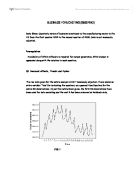
Essentially due to the seasonal factors present in the data, we need to perform the seasonal decomposition procedure to find out the SAS(Seasonally adjusted series)
We choose Analyse→Time series →Seasonal decomposition from the SPSS menu. And choose a multiplicative model type. Four new variables are created .
Sequence plot of the SAS will be like given below.
Now using the SAS data, we can perform a Linear regression analysis, which includes the three dummy variables D1, D2 and D3 for building the model.
The output is as given below
The adjusted R square gives a value of 39.2% which suggests that it is a good fit . The coefficients are given below.
From the table it is deducible that all the dummy variables are significant. So all the dummy variables can be included in the model.
A plot of the raw data and the predicted values are
So the obtained regression model will be deemed as
Investment = 5577.542 - 1080.037 * D1 - 922.571 * D2 - 665.216 * D3 – 23.466 * time + Error
We have to predict the holdback data by applying the above model. After applying the function Transform→Compute in SPSS, and entering the obtained model , the predicted model is created. The resultant predicted variables are very close to the output produced by SPSS which suggests that the predicted model is correct.
To perform an regression analysis of the dummy variable model with an non linear trend , we just have to repeat the earlier steps of the dummy variable model estimation followed by the command Analyze→Regression→Non – Linear
But when we are considering a quadratic model, we have to first create a variable using the time series function . After creating the variable we perform a non linear regression model on the data, using the three dummy variables. The output is as given below.
We find that the adjusted R square is 71.1% which suggests it is a very good fit better than linear regression model.
The coefficients of the model are
All the variables are significant
So the build quadratic model would be
Investments = 4503.761 – 1002.114 * D1 – 844.647 * D2 – 665.216 * D3 + 95.756 * time – 2.338 * + Error
So by looking at the two regression models that we have got we can see that significance factors and the adjusted R square being better for the quadratic data. So i choose the quadratic regression model be the final dummy variable model.
Q3 Box-Jenkins ARIMA model.
A Box – Jenkins model involves the analysis of the time series plot , ACF and the PACF plots of the raw data and first order differenced data.
As we have seen from our earlier analysis about the time series plot we can seemingly conclude that there is no presence of trend, but were faint seasonal factors present in the data.
The time series plots is given below
To estimate the ARIMA parameters, the trend and the seasonal patterns are to be removed from the data. For that the following two steps are made
- For the raw data the plots are seasonally decomposed , which gives the SAS variable. The seasonally adjusted data is devoid of any seasonal patterns.
- Then the Seasonally adjusted data, is differenced once to remove the trend presence and the final sequence will be devoid of any seasonal patterns, or trend or cycles
After these two major operations are made the ARIMA parameters are estimated from the ACF and the PACF plots.
The time series plots of the SAS data is as given below
Looking at the plot we can see that seasonal factors are completely withdrawn. But then there are small presence of trend and the cyclical factors, which we can remove by differencing the SAS data once. The time series plots of the differenced SAS data is given below.
The differenced time series plot clearly shows us the removal of the trend, seasonal,and cyclical pattern which can be used to make the ARIMA model now. The ACF and the PACF plots of the differenced deseasonalised data are
From the above ACF graph we can see a diminishing sine series wave, so we can say the ACF graph comes down to zero, so we need not difference the data once more . Looking at the PACF graph we can see a spike at lag 3 of the data, and then the rest of the data fall correspondingly within the confidence limits. So it could be a ARIMA(3,1,0) model for the differenced data. Or also we can fit an ARIMA(3,1,1) for the data. We can only fit and compare the models based on a lower BIC value that can be enabled from the statistics tab of the ARIMA modeller in SPSS.
Part of the SPSS output for ARIMA(3,1,0) will be
The normalized BIC value is 12.531 which we can test in comparison with the ARIMA(3,1,1) model.
Part of the SPSS output is as given below.
After seeing the normalized BIC for both the models seems to be lesser in the ARIMA(3,1,1) model , which seems to be acceptable. This model has been chosen as the best amongst all the methods by a trial and error basis. The holdback data also comes out neatly as predicted against the forecast data as indicated by the line graph. Also all the variables are within the 5% significance limit. The rest of the models are ignored but the results are separately annotated.
So the built model will be
SAF
But we know that for the raw data the equation will be
So the final built model will be like, after substituting for
Note that the seasonal factors that are removed during the beginning of the model building is multiplied back into the model at the end equation by the SAF ( Seasonally adjusted Factor)
The final phase is checking the modelling data with the holdback data which comes along with the built ARIMA model.
The modelling data seems to be fairly accurate in this case.
Q4 Differences in methods and Forms of equations used
As we have seen ,we have used two models in the analysis of our data . the dummy variable model and the ARIMA approach using the Box- Jenkins model
The dummy variable model for the linear regression has the following basic equation of
Investment = a + b1*D1 + b2*D2 + b3*D3 + c*time + Error
And for the non linear regression we get
Investment = a+ b1 * D1 + b2 * D2 + b3 * D3 + c * time + e * + Error
This equation accommodated the dummy variables D1, D2 and D3 which were entered manually in the SPSS data sheet. After which the models were predicted. Based on the fit of the data, indicated by the Adjusted R square methods , a linear regression is factored. The linear regression returned a satisfactory fit with an adjusted R square of around 39.2% which was of a good fit, but was due for a better replacement model. So a non linear regression of the quadratic form yielded a model with a better fir for the data given. The adjusted R square was 71.1%. So I took the quadratic form as my final model. Of course, if a regression of the cubic form could have yielded better results but the possibility was explored but the final results are not documented.
Predicting the holdback data, was taken as the last step of the SPSS output which can be calculated by the estimating the deviation of error variable from the main data values. In effect there was not presence of any major deviations and forecasting seemed to be of a fairly accurate measure.
The Box – Jenkins model ARIMA method yielded a final model of ARIMA(3,1,1) and the parameterized final model looked like
*SAF
The final model that i had chosen was amongst a wide range of alternatives suiting for a competing fit. But this model was chosen because it yielded the standardized results under the without any unwanted over specification and also had the lowest value of normalized BIC for similar data sets.
The forecast of the holdback data, against the full model is fairly correct as indicated by the plots of the ARIMA method.
Q5 Impact of choice of splitting the data.
As we already know, according to the question that only a part of the data a large part of the data is used in building the two models and the rest of the small part of the data is used as a holdback for testing the forecasting. The holdback data is also used in error analysis.
The in sample data set is only used to measure the goodness of the fit.The out of sample data is never really impacts the final model, but can be used to the cross verify the forecasted model.
Many of the influential observations have a great impact on the influence of the fitted equation.[Makridakis S, Wheelright S(1998)].If any of the observations are omitted from the analysis, then the acquired equation can be drastically wrong. So, utmost care must be exercised while the holdback back data is selected, so that when the data is split, it does include all the influential observations. This of course can be checked by a simple scatter plot of the raw data and deciding from which end of the spectrum to split the data ie from beginning or bottom, so that we can include the majority of the observations excluding the outliers.
In this particular question we can see that the bottom of the data with 8 observations in holdback. A simple scatter of the entire raw data might have suggested the influential observations and outliers based on which the decision is made. So to choice of where to split the data becomes essential to the analysis as a whole.
Q6 Assumptions, findings from the final model and sensitivity of the model.
A line plot of the raw data and the lagged components will provide us with an insight into the seasonal, trend and the cyclical factors. The raw data that was provided to us was analysed with scatter plots and lag 4 claimed to have somewhat resemblance to a straight line.
We know that general procedure for removal of seasonal data is seasonal decomposition and the procedure for removing the trend will be to difference the data until about when the trend factors are totally removed.
One of the major assumptions being made during the selection of dummy variables is when knowing that the data being a four point pattern repeat, the fourth dummy variable D4 is not involved in model building. This is because the inclusion would lead to similar results and thus a three part dummy variables is sufficient to build a good model. This process has been carried over to non – linear regression as well.
No irregular components are faced with during the entire stage of regression in the dummy variable model. ALL the lag values are significant in perspective and therefore none of the variables are excluded from the final model.
Similarly for the Box – Jenkins ARIMA model, both the trends and the seasonal patterns are taken out before any analysis can begin and the ARIMA model is predicted from a range of other competing models by the choice of best fit. This of course will have conflicting ideas, as most models may seem appropriate. Like I have mentioned before the choice of the ARIMA model depends upon how the ACF and the PACF graphs are going to shape up , how many factor variables are going to be significant and also how the BIC values show up on the final estimation. Finally after taking many factors into consideration it was decided to make a ARIMA(3,1,1) as the final chosen model.
Any estimation of the ARIMA with the inclusions of seasonal or trend factors will have anomalies in the final model, which shows us how these factors have an influence on the entire model.