upper quartile = L3 + [ 3N÷4−fL3 ] × C3 where L3: L.C.B. of upper quartile class
f3 N: total number of items
fL3: cumulative frequency up to pt. L
f3: upper quartile class frequency
C3: upper quartile class length
upper quartile = 20 + [ (3×100)÷4−72 ] × 5 upper quartile = 22.5
6
Interquartile range = upper quartile− lower quartile
= 22.5-14.81
=7.69
mode = L + [ Δ1 ] × C where L: L.C.B. of modal class
Δ1+Δ3 Δ1: difference in frequencies between modal
class and pervious class
Δ3: difference in frequencies between modal
class and following class
C: width of modal class
mode = 15 + [ 20 ] × 5 mode = 16.67
20+40
standard deviation = ∑ƒx − ∑ƒx
∑ƒ ∑ƒ
standard deviation = 63925 − 2210 standard deviation = 12.28
100 100
Standard deviation can be thought of as a measure of average dispersion about the mean. Hence the smaller the value of the standard deviation, the closer the data is to the mean. The value of the standard deviation of the height of the birds is very large, which means the data is spreaded throughout the distribution. (this is also shown in the box-and-whisker plot).
This information can be used to plot a histogram and from that, I can also identify whether the distribution has a positive or a negative skew. From the histogram, I can easily state the modal group of the data, however, as the data is grouped in class intervals, an exact single value can not be found from it.
Mean Average Deviation = ∑ƒ⏐x − x ⏐
∑ƒ
mean deviation = 922.4 mean deviation = 9.224
100
Data Presentation for Analysis
Calculation:-
mean = ∑ƒx mean = 4080 mean = 40.8
∑ƒ 100
median = L+[ N÷2−fL ] × C where L: L.C.B. of median class
f N: total number of items
fL: cumulative frequency up to the point L
f: median class frequency
C: median class length
median = 30 + [ 100÷2−38 ] × 5 median = 31.71
35
lower quartile = L1+ [ N÷4−fL1 ] × C1 where L1: L.C.B. of lower quartile class
f1 N: total number of items
fL1: cumulative frequency up to pt. L
f1: lower quartile class frequency
C1: lower quartile class length
lower quartile = 20+ [100÷4−5 ] × 5 lower quartile = 23.03
33
upper quartile = L3 + [ 3N÷4−fL3 ] × C3 where L3: L.C.B. of upper quartile class
f3 N: total number of items
fL3: cumulative frequency up to pt. L
f3: upper quartile class frequency
C3: upper quartile class length
upper quartile = 40 + [ 3×100÷4−73 ] × 5 upper quartile = 41.11
9
Interquartile range = upper quartile− lower quartile
= 41.11− 23.03
= 18.08
mode = L + [ Δ1 ] × C where L: L.C.B. of modal class
Δ1+Δ3 Δ1 : difference in frequencies between modal
class and pervious class
Δ3 : difference in frequencies between modal
class and following class
C: width of modal class
mode = 30 + [ 2 ] × 5 mode = 30.36
2+26
standard deviation = ∑ƒx − ∑ƒx
∑ƒ ∑ƒ
standard deviation = 223300 − 4080 standard deviation = 23.84
100 100
The value of the standard deviation is very high for the length of the birds’ wing-spans. This suggests that this set of data is widely spreaded throughout the distribution.
Interpretation:-
The two cumulative frequency graphs (one for the height of the birds and the other one for the length of the birds’ wing-span ) show a similar pattern in terms of their shapes. The gradient, where it is at its steepest, represents the mode of the data. On both graphs the steepest gradients of the curves lie within the median and the lower quartile of both data. By using calculations, the mean of the height of the birds works out to be 22.1cm; and the mean of the length of the birds’ wing-span is 40.8cm. These two values seem quite reasonable for a bird’s body measurement and they are the average values of the data that I collected.
The calculations of the medians, the lower quartiles and the upper quartiles match the values that are shown on the two cumulative frequency graphs. This suggests that they are calculated to a certain degree of accuracy and the readings from the graphs are just as accurate as the calculated ones, although the graphs may not be able to give exact values. The standard deviation shows how spread out the data is. The larger the value, the greater the spread of the data is. In this case, both standard deviations turn out to be very large, which means both dispersions of the two sets of data are quite similar in terms of how spread out the data is.
Probability:-
To find out if the two events are independent or mutually exclusive, the following calculations have to be done.
P(A) = probability of choosing a data from the median class of the set of data that shows
the height of the birds.
P(B) = probability of choosing a data from the median class of the set of data that shows
the length of the birds’ wing-span.
P(A) = 46 P(B) = 35
100 100
If the two events (A and B) are independent then P(A⎜B) = P(A) or P(B⎜A) = P(B).
P(A⎜B) = P(A∩B) P(B⎜A) = P(B∩A)
P(B) P(A)
= 0.161 = 0.161
0.35 0.46
= 0.46 = 0.35
Now P(A⎜B) = 0.46 and P(A) = 0.46 which means the two events are independent.
And P(B⎜A) = 0.35 and P(B) = 0.35 which shows the 2 events are definitely
independent.
This suggests that whether the chosen data is from the median class of the birds’ height or not P(A), it would not in any way influence the probability of getting a data that is from the median class of the other set of data P(B).
If the two events are mutually exclusive, P(A⎜B) = 0
But now, P(A⎜B) = 0.64 which does not equal 0.
This shows that the two events are not mutually exclusive, which means they can happen at the same time.
The probability of selecting a data from the median class of both sets of data is:
P(A) = probability of choosing a data from the median class of the set of data that shows
the height of the birds.
P(B) = probability of choosing a data from the median class of the set of data that shows
the length of the birds’ wing-span.
P(A) = 46 P(B) = 35
100 100
P(A∩B) = 46 × 35
100 100
= 0.161
The probability of choosing a data from the median class of either set of data is:
P(A∪B) = P(A) + P(B) − P(A∩B)
= 46 + 35 − ( 46 × 35 )
100 100 100 100
= 0.649
From the probability calculation above, it shows that the probability of choosing a data that is in both median classes has a less chance of success than choosing the one that is in either of the median classes of the two sets of data.
Interpretation:-
From the probability calculation above, I can establish that the two sets of data that I collected are not mutually exclusive but are independent. It relates to the aim of my investigation which is stated in the introduction. As known from the fact, the larger the bird, the larger the wing-span it would have. The average height and the wing-span that are calculated seem quite reasonable. From the interquartile range, I can see a much better measure of spread than the range ( which is just simply taken the lower extreme and subtracts it from the upper extreme; as the differences of these two values of both sets of data are quite large, the range would not give a very accurate measure of the spread.).
The histogram shows clearly the modal group of the data. It is often a very quick way of finding the modal group of a certain data, but it cannot give an exact value, so to calculate the mode I used the formula which gives a more precise answer. The box-and-whisker plot works just as well as the cumulative frequency graph. However, before drawing the box-and-whisker plot, the median, the lower and the upper quartiles must be worked out. Otherwise, the quartiles and the median can be just read off from the cumulative frequency graph. Both ways of presenting the data are just as good, as long as the calculations are done before drawing the box-and-whisker plot. From the cumulative frequency curve, I can also work out the percentage of the data that lies within the range called “mean ± 2 standard deviation”. This range is to show how the data is spreaded out about the mean, and from that I can also calculate the percentage of the data that falls into the category of outlier.
When grouping the data, I have used two methods. One is using a Tally Chart and the other one is using a Stem and Leaf diagram. Both methods are a quick way of grouping data, but the stem and leaf diagram seems to be more useful because the original values are not lost when the data is grouped. I have chosen to use these two different methods because they show me the advantages and the disadvantages within them. In comparison, using the stem and leaf diagram is just slightly more time consuming than using the tally chart. That’s because that figures have to be noted down and best to place them in order so that it would seem more logical.
Evaluation:-
Although the data is collected in a large quantity, but the values of which seem to be very small and crowded together. This would affect the values of the mean, the median, the mode and the interquartile range. The data takes in an account of a wide range of birds’ species, however, the data happens to be restricted to small measurements. Therefore the mean, median and the mode cannot represent the average body measurement of birds in the world. However, they can represent the average body measurement of birds that are within the height of 10-90cm and the wing-spans’ length of 10-90cm.
Although the data is selected randomly from the three different reference books, but the data still has a restriction ( limited to small values) within itself. If I have to do this investigation once more, when I am collecting the data, I will ensure that it includes a wide range of measurements so that it can be a representative of most of the birds in the world. Apart from that, I will also look into other reference books about birds that are from all over the world; rather than only just the books that include the birds in Europe, the Middle East and North Africa. In this way, I may be able to get more data of different birds and their body measurements will vary more. The calculations that are using this data can be more of a representative of the averages of the birds from all over the world.
If the data is of a wider range, I can calculate it to see if it is a binomial distribution
or not. It can also help me to carry out a hypothesis testing for the binomial distribution. Pie charts can also be drawn to present the data if it has a wide range of measurements ( in terms of the height of the birds and the length of the birds’ wing-span ). The probability of a certain event occurring can also be calculated and compares to the probability that is calculated using the data that I have got now.
Personally, I am quite interested in birds and this investigation can help me to increase my knowledge of this subject and therefore I can have a deeper understanding about different species of birds in the world.