The value of parameter could be determined algebraically by determining the period, which is 365 days. The period is then used with the value 2π (the period of a sinusoidal function is , so the period equals to 365). Therefore, the equation should be = , which results in the answer 0.017.
5. Use a sinusoidal regression to find the equation, in the form g(n) = a sin[b(n – c)] + d, that represents the time of sunrise as a function of day number, n, for Miami. State the values of a, b, c, and d to the nearest thousandth.
The values of the parameters a, b, c, and d to the nearest thousandth are:
a = 0.846
b = 0.015
c = 127.798
d = 6.362
The equation that represents the time of sunrise as a function of day number, n, for Miami through sinusoidal regression is g(n) = 0.846 sin[0.015(n –127.798)] + 6.362. This is found through using the TI-84 Plus graphing calculator. All the coordinates are listed in a table and the equation is found using sinusoidal regression, which is done with the graphing calculator.
6. State the range, domain, and period of the function representing the time of sunrise for Miami that you found in question 5.
The domain of the function would be {x Є R | 1 ≤ x ≤ 365} and the range of the function would be {y Є R | 5.516 ≤ y ≤ 7.208}. The period of the function representing the time of sunrise for Miami is , which results in the answer 0.017. The domain represents the number of days, starting from day 1 to day 365, since day 0 does not exist. As a result, the domain is equal or in between 1 and 365. The range of the function represents the time of sunrise. Therefore, the minimum and maximum values are found out, equal or in between 5.516 and 7.208. The period of a sinusoidal function is , so the period equals to 365 (there is 365 days in a year). Therefore, the answer becomes , which is 0.017.
7. The graph of function f, which represents the time of sunrise in Toronto, can be transformed to the graph of function g, which represents the time of sunrise in Miami. One of the transformations that occurs is a vertical stretch. Calculate the vertical stretch factor that would be required in the transformation of the graph of function f into the graph of function g.
The amplitude that represents the time of sunrise in Toronto is 1.627 and the amplitude that represents the time of sunrise in Miami is 0.846. A certain value, which is the vertical stretch factor, must be multiplied by 1.627 in order to get the value of 0.846.
Let a be the vertical stretch factor.
1.627 a = 0.846
a =
a = 0.520
The vertical stretch factor that would be required in the transformation of the graph of function f into the graph of function g would be 0.520.
Part B
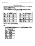
1. Use the data in the list of sunrise times and the data in the list of sunset times for Toronto to create data for a new list that shows the number of hours of daylight for the 12 dates given. Use a sinusoidal regression to find the equation for the number of hours of daylight as a function of the day number, n, for Toronto.
Write your equation in the form T(n) = a sin[b(n – c)] + d, with a, b, c, and d rounded to the nearest thousandth.
The times of sunrise and sunset for Toronto are converted to a decimal and they are all placed on separate charts. All of the data from the two charts are used to created a chart that states the number of hours of daylight for the 12 dates given.
The values of the parameters a, b, c, and d to the nearest thousandth are:
a = 3.255
b = 0.017
c = 78.351
d = 12.119
The equation for the number of hours of daylight as a function of the day number, n, for Toronto through sinusoidal regression is T(n) = 3.255 sin[0.017(n – 78.351)] + 12.119. This is found through using the TI-84 Plus graphing calculator. All the coordinates are listed in a table and the equation is found using sinusoidal regression, which is done with the graphing calculator.
2. Repeat the procedure above to find the equation for the number of hours of daylight as a function of the day number, n, for Miami. Write your equation in the form M(n) = a sin[b(n – c)] + d, with a, b, c, and d rounded to the nearest thousandth.
The times of sunrise and sunset for Miami are converted to a decimal and they are all placed on separate charts. All of the data from the two charts are used to created a chart that states the number of hours of daylight for the 12 dates given.
The values of the parameters a, b, c, and d to the nearest thousandth are:
a = 1.611
b = 0.017
c = 78.843
d = 12.114
The equation for the number of hours of daylight as a function of the day number, n, for Miami through sinusoidal regression is M(n) = 1.611 sin[0.017(n – 78.843)] + 12.114. This is found through using the TI-84 Plus graphing calculator. All the coordinates are listed in a table and the equation is found using sinusoidal regression, which is done with the graphing calculator.
3. Using a GDC or graphing software, graph the functions T(n) and M(n). Choose an appropriate scale, and sketch the graph of each function on a single grid.
All the values of the number of hours of daylight, both Miami and Toronto, are listed into Microsoft Excel. The two functions are graphed onto one single grid, in which the blue line represents the number of hours of daylight in Toronto and the pink line represents the number of hours of daylight in Miami. Everything on the graph is labelled.
4. Determine the number of hours and minutes of daylight in Toronto and Miami on May 24 (day 144).
Substitute 144 into n in the function T(n).
T(n) = 3.255 sin[0.017(144 – 78.351)] + 12.119
T(n) = 3.255 sin[0.017(65.649)] + 12.119
T(n) = 3.255 sin(1.116033) + 12.119 (use radian mode)
T(n) = 2.924178114 + 12.119
T(n) = 15.04317811
T(n) = 15 hours and 3 minutes
Substitute 144 into n in the function M (n).
M(n) = 1.611 sin[0.017(144 – 78.843)] + 12.114
M(n) = 1.611 sin[0.017(65.157)] + 12.114
M(n) = 1.611 sin(1.107669) + 12.114 (use radian mode)
M(n) = 1.441296853 + 12.114
M(n) = 13.55529685
M(n) = 13 hours and 33 minutes
The number of hours and minutes of daylight in Toronto on day 144 is 15 hours and 3 minutes and the number of hours and minutes of daylight in Miami on day 144 is 13 hours and 33 minutes.
5. Explain how the latitude of a location is related to the hours of daylight, and explain how this relationship is illustrated by the differences in the parameters in the two equations.
The latitude of a location is related to the hours of daylight, since there are more hours of daylight and a smaller range between the smallest number of hours of daylight and greatest number of hours of daylight as you go south towards the equator. This relationship is illustrated by the differences in the parameters in the two equations, since a, which is the amplitude of the function, is higher in Toronto (3.255) than Miami (1.611). This shows that there is a higher maximum value, as well as a lower minimum value than Miami, which results in a higher amplitude. For the parameter b, the values are the same, since the period is for both functions, which equals to 0.017. For the parameter c and d, the values are almost the same, since the phase shift, which is very close to the longitude of the two cities, since they move at the same degree from the equator. The vertical shift would approximately show the mean number of daylight numbers of the two cities, since a sine function usually starts at the mean value, goes to the maximum value as the x-value increases, and returns to the mean value (and it continues on). As a result, these two values form a coordinate (c, d), which is extremely close to the first point of intersection between the two sinusoidal functions.
6. One factor that affects a region’s growing season is hours of daylight. Toronto’s growing season generally starts when there are 15 or more hours of daylight per day. If this were the only factor, then what would be the predicted start date and end date of the growing season in Toronto? Explain the method you used to determine these dates.
The predicted start date and end date of the growing season in Toronto would be Day 143 and Day 200. The method that is used to determine these dates is through using the TI-84 Plus graphing calculator. The sinusoidal function T(n) = 3.255 sin[0.017(n – 78.351)] + 12.119 and the line y=15 are put onto the graphing calculator. A graph is drawn from the two equations and the points of intersection are found out using the graphing calculator. Another way is to find the start date and end date algebraically.
7. Explain how functions T and M, which you determined in part B, questions 1 and 2, could be used to determine the days on which Toronto and Miami have the same number of hours of daylight. Explain the method you would use to determine these dates.
The functions T and M could be used to determine the days on which Toronto and Miami have the same number of hours of daylight by putting the two equations on a single grid and find the points of intersection. The method that I would use to determine these dates would be to insert the equations T(n) = 3.255 sin[0.017(n – 78.351)] + 12.119 and M(n) = 1.611 sin[0.017(n – 78.843)] + 12.114 into the TI-84 Plus graphing calculator. Then, a graph would be drawn from the two equations and the points of intersection would be found out using the graphing calculator. As a result, there are two points of intersection that are seen on the grid. The two days on which Toronto and Miami have the same number of hours of daylight are Day 78 and Day 263.
8. Using the data that you obtained for the number of daylight hours per day in both Toronto and Miami, complete the following table
Mean number of daylight hours for Toronto
= 12.21h
Mean number of daylight hours for Miami
= 12.15h
Which parameter, a, b, c, or d, in functions T and M is most closely related to the mean number of daylight hours. Explain your answer.
The parameter d is most closely related to the mean number of daylight hours in functions T and M, since it is the mean value of the sinusoidal graph, which is extremely close to the mean number. It represents the mean number, since the mean number would approximately equal to the vertical shift if n is the value of the phase shift.
9. For Miami, consider June 21 (day 172), with 13.72 hours of daylight, as the day on which there is the maximum number of hours of daylight and December 22 (day 356), with 10.51 hours of daylight, as the day on which there is the minimum number of hours of daylight. Using the data from these days (not the regression data), algebraically determine a cosine equation in the form of h(n) = a cos[b(n – c)] + d for the number of hours of daylight. Explain how you determined each of the parameters, to the nearest thousandth, of h(n) = a cos[b(n – c)] + d. Comment on how well your function fits the data.
In order to figure out the cosine equation, we must figure out all the parameters in the equation.
a = == 1.605
b = = 0.017
d = = = 12.115
In order to find out the entire cosine equation, we must substitute in one of the coordinates into the equation in order to find the value of c.
h(n) = a cos[b(n – c)] + d
13.72 = 1.605 cos[0.017(172 – c)] + 12.115
1.605 = 1.605 cos[0.017(172 – c)]
1 = cos[0.017(172 – c)]
0 = 0.017(172 – c)
0 = 172 – c
-172 = - c
c = 172
Therefore, the cosine equation in the form of h(n) = a cos[b(n – c)] + d for the number of hours of daylight that is algebraically determined is h(n) = 1.605 cos[0.017(n –172)] + 12.115.
The function fits extremely well into the data, since both functions look extremely identical to one another. All the coordinates fit in together and the graph looks like one grid with two unison sinusoidal functions. This shows that the cosine equation is extremely accurate, since it fits exactly on the graph shown on the TI-84 Plus graphing calculator.