Common sense says that a firm will tend to buy labour if the added benefit to the firm (the Marginal Revenue Product) exceeds the added cost (Marginal Resource Cost). The added benefit is the value to the firm of the extra output which the hours of labour produces. If increasing the amount of the hours of labour raises revenues more than it raises costs, a firm can increase its profits by using more labour this is the case of MRP exceeding MRC. If reducing the amount of hours of labour cuts costs by more than it cuts revenues, a firm can increase its profits by using less labour This is the case of MRC exceeding MRP, It follows that if the firm has maximized profits, MRP must equal MRC. If the firm should increase resource use when MRP exceeds MRC, and if it should decrease resource use when MRP is less than MRC, then it is using just the right amount when MRP equals MRC.
To push the analysis further, assumptions that many firms buy labour expecting to change price within the market, but none can noticeably influence price in any market. This assumption that firms are means that marginal revenue equals price of output, and that the marginal resource cost equals the price of the resource.
With these assumptions, a diagram similar of economic efficiency. On the left we have a representative worker who sells hours of unskilled labour. The supply curve is drawn so that it slopes upward. To find the market supply curve, you must add up all the hours of work which will be offered at each wage.
On the right we have buyers of unskilled labour. Its demand curve will be the downward sloping part of its MRP curve. The MRP curve is the demand curve for labour because this curve tells how valuable another unit of the resource is to the firm. Hence, given a wage, one can tell how much labour a firm demands by looking at the MRP curve.
To find the market demand, one must add up at each wage the number of labour hours demanded by each firm. The intersection of the market demand and market supply curve gives the equilibrium wage, it will hire all workers who contribute more to the firm than they cost.
There are some important results which come from this simple analysis. First, owners of resources are paid their marginal contribution to output. An owner of a resource which adds a more valuable contribution to output is paid more than an owner of resource which adds a less valuable contribution. . For example, rubbish collectors perform a vital service in large cities, and when they go on strike, people are not only tremendously inconvenienced, but their health may be threatened. The total value of the services of garbage collectors is very high. But this high total value does not mean that the value of another rubbish collector is high. If adding or removing one rubbish collector changes the value of rubbish collection services little, then this marginal contribution will give a low wage in this market.
The graphs above can help illustrate changes which will raise or lower wages or other payments to inputs. There are two reasons the demand curve could shift. First, it could shift because people value the output more. For example, the high salaries of professional football players are due to the popularity of football as a spectator sport. A century ago a man with the same abilities of David Beckham or Michael Owen would have earned a normal income because there was no demand for his special talents.
Second, the demand curve could shift because of increased productivity, perhaps caused by changes in the amounts of other resources. A trend in industrialised societies has been to replace physical work with machines. As a result, the rewards going to muscle power have fallen as compared to the rewards going to brain power.
The supply curve can also change, and as it does, so will the income which the resource earns. A new discovery of metal ore will reduce the value of known deposits. Increased availability of education increases the numbers of doctors, lawyers, teachers, and accountants. If demand for their services does not change, their increased numbers will cause their incomes to drop. People who want to control the wages they earn have usually curve.
Adding together all buyers and sellers of unskilled labour, or aggregating them, is useful because it gives us insights. Sometimes extreme aggregation is useful, such as treating all labour services in the same market. This sort of extreme aggregation is . In the case of labour markets, such aggregation is useful if we slightly alter our graph above
Equilibrium in the labour market requires that MRC=MRP. With the assumption that everyone is a price taker, this condition can be written as:
(1) Marginal Product x Price = Wage.
If both sides are divided by price, we get:
(2) Marginal Product = Wage/Price = Real Wage.
The , or wages divided by prices, measures the purchasing power of what workers earn.
The illustration below graphs the marginal product of labour and the supply of labour as a function of the real wage. Suppose the amount of labour declines. The supply curve will shift to the left, the marginal worker will become more productive, and the real wage will rise. Labour will become scarcer relative to land and equipment, which have not changed. The Black Death in 14th century Europe reduced population by about 30% in a few years. As the illustration suggests, real wages rose as a result.
The graph also suggests why economists in the 19th century so often saw as a way to solve poverty. Fewer people will, other things held equal, increase wages and more people will reduce them. However in the real world those other factors have often not remained equal. Europe is densely populated and Africa is sparsely populated, yet Europe has a vastly higher standard of living than Africa.
Economic theory traditionally explains income differences in terms of . If we have a mason who can lay 50 bricks and hour, we expect him to earn twice as much as the mason who can lay only 25 bricks per hour because if any other wage rate existed, there would be a profit opportunity for building contractors. If the more productive mason works for less than twice as much as the other, everyone would want to hire him and no one would hire the less productive one. Only when his wage is exactly twice as high, exactly paralleling the difference in productivity, would people be equally willing to hire either.
This way of explaining wage differentials suggests that the very large differences in income are the result of equally large differences in performance. However, there is an alternative explanation which says that in many cases relative differences in performance, not the absolute differences, determine earnings. This explanation of wage differences in terms of relative performance is often called tournament theory. One place where this explanation should work is in contests with winners and losers. For example, consider two almost equally able gladiators fighting in the arena of ancient Rome.
Another place where relative ability may matter a great deal is in the managerial ranks of corporations. There are limited numbers of promotions available, and they are usually determined by relative performance. Only one person can be CEO of a company at a time, and small differences in ability among those contending for the top spot can result in large differences in rewards. Further, it may be in the interests of the company to structure pay so that the winner makes very large sums as a way of spurring on those lower in the hierarchy. The primary reason for the high pay given to the CEO may be to give those lower in the hierarchy an incentive to work hard, not to give the CEO himself the incentive to perform well.
The argument that winner-take-all contests tend to over-attract entrants closely parallels the argument that the : people respond to average benefit rather than to marginal benefit.