I will consider the variables as a sequence, and from there I shall calculate the polynomial equation modeling this situation.
First I will find the pattern in the sequence. To find the pattern, I will list the numbers, and find the differences for each pair of numbers. That is, I will subtract the numbers in pairs (the first from the second, the second from the third, and so on), like this:
10 23 38 55 74 96 120 149
13 15 17 19 22 24 29
Since these values, the "first differences", are not all the same value, I'll continue subtracting:
10 23 38 55 74 96 120 149
13 15 17 19 22 24 29
2 2 2 2 2 5
Since these values, the "second differences", are all the same value, then I can stop. It isn't important what the second difference is (in this case, "2"); what is important is that the second differences are the same, because this tells me that the polynomial for this sequence of values is a quadratic. Since the formula for the terms is a quadratic, then I know that it is of the form:
ax2 + bx+ c
Note: The quadratic function applies until the 7th guide. Since there is a difference of “5” between 29 and 24 instead of being “2”.
Now I have to fine the value of the coefficients, a, b and c. In order to calculate these I’ll plug in some values from the sequence, and then solving the resulting system of equations. For instance, I know that the first term (where n = 1) is 10, so I’ll plug in 1 for n and 10 for the value:
a(1)2 + b(1) + c = a + b + c = 10
The second term (that is, the term when n = 2) is 23, so:
a(2)2 + b(2) + c = 4a + 2b + c = 5
The third term (that is, the term when n = 3) is 38, so:
a(3)2 + b(3) + c = 9a + 3b + c = 38
This gives me a system of three equations with three unknowns, which I can solve.
a + b + c = 10
4a + 2b + c = 23
9a + 3b + c = 38
I used a graphical display calculator to calculate the value of a, b and c.
The method which I used in the GDC was using “simultaneous” equation solver. The results I obtained were as follows:
a = 1
b = 10
c = -1
Hence the quadratic function is
Another method which I used to find the Quadratic function was using a software called Ms.Excel.
A quadratic function is expressed in the form of. The values of the coeffients a, b, and c was found to be:
a = 1.214
b = 8.738
c = 0.464
Hence, the Quadratic function that models this situation is y = 1.214x2 + 8.738x + 0.464.
In order to find a cubic function to model this situation the same software was used.
A cubic function is expressed in the form of. The values of the coeffients a, b, c, and d was found to be:
a = 0.055
b = 0.464
c = 11.59
d = - 2.285
Hence, the Cubic function that models this situation is y = 0.055x3 + 0.464x2 + 11.59x - 2.285
The graph below shows the two functions plotted on one set of axes.
The difference between the two functions is not much. However the quadratic function fits a simple curve to the data points, and when we increase the order of the equation to a third degree polynomial (cubic function), it forms a curve through those data points also, but is slightly lower than the quadratic function.
In order to find a polynomial function that passes through every data point, I have used the same software as above. The polynomial function is to a fourth degree polynomial.
A quartic function is expressed in the form of. The value of the coeffients a, b, c, d and e was found to be:
a = 0.020
b = -0.319
c = 2.729
d = 6.402
e = 1.25
Hence, the Quartic function that models this situation is y = 0.020x4 - 0.319x3 + 2.729x2 + 6.402x + 1.25
The graph below, shows a comparison if all the three polynomial functions.
Again there are not many differences between the three functions. The cubic function bends more lower down than the other two. The Quartic Function passes through all the data points in a smooth curve almost like the Quadratic Function.
I believe that the function which best models this situation is the quadratic function. I chose this equation because it forms a smoother curve which passes through all the data points. Also, using the sequence and Pattern method, it justifies that the data forms a quadratic function.
Using my Quadratic model, I’ll decide where I could place a ninth guide. My Quadratic Function was
y = 1.214x2 + 8.738x + 0.464. In order to find the distance of the guide from the tip, I will substitute x with 9 in the equation. 9 is the guide number. I get y (distance from the tip) to be equal to 177.44 cm, which is approximately equal to 178 cm. Adding a ninth guide, forms a curve which is shown below:
If I compare this curve, with the original curve of 8 guides, we can see that the new curve is slightly steeper than the second curve.
Hence, I consider that the implication of adding a ninth guide to the fishing rod is a good one. This is because the last guide (9th guide) is closest to the reel. It allows the line to come off the pool much easier. Basically to sum it up, the more guides the more line control, and hence the farther and smoother the cast, giving a smoother retrieve.
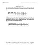
Table 2, shows the distances for each of the line guides from the tip of Mark’s fishing rod.
Table 2
The graph below shows how well my quadratic model fits this new data:
As we can see, Mark’s fishing rod’s set of data points forms a less steep curve than Leo’s fishing rod.