b= 2 - 3(0.5)
b= 2 – 1.5
b = 0.5
Now, by combining the values of a and b, we can derive a general statement for the nth term of the numerator (where n is the row number) :
To prove the validity of this statement, I will use the 5th row with 15 as the numerator number (n):
N = 0.5(5) 2 + 0.5(5)
N = 12.5 + 2.5
N = 15
Another way to prove that the general statement of finding the numerator is correct is by using technology. In order to find out which trendline best fits the data in Table 2, I will be plotting different trendlines on Microsoft Excel and analysing the coefficient of determination. The coefficient of determination, known as R2, is used to determine how well future outcomes are likely to be predicted using the model on the basis of related information.
The value of R2 ranges from 0 to 1 with 1 representing the most accurate value. As the value of R2 of a certain model gets closer to 1, it becomes a better representative of the future data trends. So the closest R2 value to 1 will be the best model of the data.
Table 2
Graph 1: Row number against numerator with a linear trendline
Graph 2: Row number against numerator with an exponential trendline
Graph 3: Row number against numerator with a polynomial trendline
Out of the three trendlines used to represent data from Table 2, the polynomial function is the best-fit model. This is because the R2 value is exactly 1, meaning that there are no other functions that can be a better fit to this data set. A polynomial equation is equal to a quadratic equation when it is to the power of 2. Since this model fits perfectly, it therefore shows a quadratic equation. Also, the equation of the polynomial trendline (Graph 3) is y= 0.5x2 + 0.5x + (4x10-14). This equation is very similar to the one derived using the simultaneous equations, only that the equation I derived doesn’t have the 4x10-14. The value of 4x10-14 is too small to make any significant influence over the equation. This reinforces that the graphing method using Excel and the equation found using algebra is the same. Thus this means that the equation for the nth term for the numerator is correct.
Finding the general statement for denominators
After finding the numerator values and the general statement for it, we also have to find a general pattern statement for the denominator values. The given triangle in Figure 1 is symmetrical. This means that the numbers on the left are identical to the ones on the right. I will be considering the relationship between the numerator and denominator.
The denominators will be categorized into different elements (as shown in Figure 3) and analysed individually.
The tables below show the relationships between the row number (n) and the difference between the numerator and denominator. The 1’s at the start and end of each row will not be used in this particular investigation, as it is not a fraction.
Table 3
For element 1, the difference between the numerator and the denominator increases steadily by 1. This means that the number always has to be subtracted from the numerator to attain the denominator. Looking at the relationship between the row number and the difference between the numerator and denominator in Table 3, there is clearly a difference of 1 between the two. This pattern initiates the following equation (where n equals the row number):
Denominator = Numerator – 1(n – 1)
Table 4
For element 2 of Lacsap’s fractions, the differences are increasing by multiples of two. This means that everything has been doubled; therefore another equation can be deduced:
Denominator = Numerator – 2(n – 2)
Table 5
Again with element 3, the differences are increasing by multiples of 3. So the equation gained from element 1 has to be tripled. This produces the following equation:
Denominator = Numerator – 3(n – 3)
Looking at the three equations derived above, there is an emergence of a pattern. The numbers in each equation match up to their element number hence they are substitutable. Using the format of the first equation deduced from element 1, the element number (r) could be substituted for 1. This results a general statement for the nth term of the denominator where D is the denominator and N is the numerator:
D = N –r(n – r)
or
The general statement for En(r)
We have now obtained the general formula for both the numerator and denominator values. Both these formulas can be combined to form a general statement.
=
Finding the sixth row
The general statement will firstly be used to find the sixth and seventh rows. To find the sixth row, the row number will be inputted for n and the element will also be inputted for r. The working is shown in Table 6.
Table 6: Calculating the values on the sixth row
As mentioned before, the “1’s” were discarded whilst doing the investigation, but now it must be added back into the beginning and end of the row. Using the calculations from Table 6, the entire sixth row is shown below:
Finding the seventh row
Likewise, the seventh row is also found by doing the same calculations as above, only this time the row number (n) will be 7. The calculations are presented in Table 7.
Table 7
The seventh row comes out as the line below:
Testing the validity of the general statement
To test the validity of the general statement, I will use the statement to find additional rows. By using the same method to finding the sixth and seventh row, the eighth and ninth row will also be calculated.
Table 8 shows the calculations for finding the values in the eighth row.
From the calculations, the eighth row will look like the following:
Moving on to solve the ninth row to further validate the generate statement. Table 9 shows the calculations for the values of row nine.
Table 9
Therefore, the ninth row will look like this:
From solving the eighth and ninth row, we can prove the validity of the general statement. The numerators calculated using the statement can be reinforced using Figure 1, Pascal’s triangle. As for the denominator, because of the symmetry observed and the pattern of the difference between the numerator and denominator is still existent. This proves that the general statement is valid and will continue to work.
Limitations
However, there are some limitations to the general statement produced. Firstly, the statement is only valid when n ≥ 1. This also means that the value of n cannot be a negative number due to the fact that any negative number when squared will equal to a positive value. The same limitations apply to the value of r, which has to be greater than zero (r ≥ 1) and an integer (ℤ) as it is not possible for a negative or incomplete element to be in the pattern. Hence, the general statement will be limited to numbers from the set of natural numbers (ℕ). Also, 0 rows does not make practical mathematical sense so it can also be regarded as a limitation to this task.
During the investigation, the “1’s” at the beginning and end of each row did not count when making calculations, as they were not proper fractions. This indicates that the 1st element of each row was actually the second number because the “1’s” were not included. Therefore there is a limitation to my general statement, as it cannot be used to calculate anything in the first row of Lacsap’s fractions in Figure 1 because that row only has two 1’s.
As Lacsap's Fractions are a sequence, sequences can be finite and infinite. We based the whole general statement on the condition that the pattern observed from the fifth row will continue infinitely. Therefore we can only assume that from extrapolating the data given, we find a common 2nd difference. The pattern for the numerator is also only based on a theory that it falls into a quadratic pattern and that it is a perfect math model when plotting the graph. The general statement only allows us to test up to a certain amount We cannot test infinite number of rows based on the general statement so there is not way to be certain whether there will be a chance of randomness in the sequence.
Conclusion
I have concluded with my general statement through a process. Firstly, I found the general statement for the numerators in each row through observations and calculation through simultaneous equations. This was then validated through the use of Microsoft Excel. To find the pattern for the denominator, I noticed a relationship between the numerator and the denominator. By splitting the elements and using the differences as a base, I noticed that the general statement for the denominator also had a correlation with the element number and row numbers. This allowed me to calculate a general statement for the denominator pattern. With both the statement for the numerator and the statement for the denominator, I was able to combine them to form the general statement, En (r).
Figure 4 is a newly devised figure of Lacsap’s fractions that has all the values up to the 9th row Through Pascal’s triangle numbers, the use of graphing technology, the observation of symmetry for the denominator, I have drawn to the conclusion that my statement is valid for all the values I have calculated and tested.
Image taken from <http://www.janak.org/pascal/pascal1.html>, November 12th 2012