Guestimate - investigate how well people estimate the length of lines and the size of angles.
Guestimate - Statistics Coursework
We have been given a piece of Statistics coursework called 'Guestimate', that asks us to investigate how well people estimate the length of lines and the size of angles. I started my investigation by creating these 3 hypothesis:
. Students in year 10 estimate angles better than students in year 7.
2. The population find it easier to estimate horizontal lines than diagonal lines.
3. The population estimate the length of lines more accurately than the size of angles.
I tried to choose three different hypotheses to avoid sticking to one particular topic. These are my reasons for choosing each of my hypothesis:
. Year 10 students have been studying angles longer than year 7 students and should be more conscious of the subtle differences between them. Also they will recognise obvious angles such as 90 degrees and use them as a base for other angles close to them.
2. Horizontal lines are seen and used more often than diagonal lines. They also look shorter than diagonal lines and are easier to estimate because of this.
3. People draw lines more often than uncommon angles (angles that are not 90, 360 or 45 degrees) and will be better at estimating something familiar.
There is a total number of 360 students in year 10 and 7.This is too large a population to collect data from, so I will take a smaller sample of 30 students from each year. There are 2 ways to select the samples:
. Stratified random sampling - This is when the population is arranged in their sets before a random sample of each set is taken according to this rule: number in set x 30 = number of students from that set
Number in year
2. Systematic Random Sampling - This is when you have a numbered list of the population before you and throw a dice to determine which number student you start on. You continue counting in this number until you have your total sample. Note down the name and number of each student you pick. A rule for this could be: "Select every 5th name on the list for your sample."
This is all good so far, but there is the very big problem of bias. To avoid bias I will not pick angles such as 90, 45 and 60 degrees as these are obvious angles and can be guessed easily. They are usually taught before doing anything else on angles. I also will not pick angles ending in 5 or 0 as these can be obvious as well and many people assume that they will end with one of the above. Furthermore, some year 7s make right angles with their thumb and index finger, so this is another reason not to pick obvious angles. To prevent this I am saying that they are not allowed to use their hands in that way, or to touch the paper other than holding it. With lines, I am not choosing whole numbers like 8cm, as these are very obvious and easy to estimate. I will use numbers like 8.4cm to make it harder to estimate. I will not choose numbers like 7.5cm either, because they are halves and are easy to estimate. I will only choose numbers with one decimal place because that way it isn't too hard to guess. I chose the angles 127 degrees for my obtuse angle and 33 degrees for my acute angle. I thought it was a good idea to pick one of each type of angle to make sure that I didn't bias my results by picking the same type of angle. I have chosen the length 6.2cm for my lines. I'm using the same length of lines because I don't want to change more than one variable as this could jeopardize whether or not my test is biased. I am putting one line horizontally on the page and one diagonally.
There is also a form of bias from using systematic random sampling. This is that I could end up with my entire sample being in one set, which could influence my results substantially. However this is very unlikely that every 5th student would be in set 1, but I would rather not take any chances. Because of this I am using Stratified random sampling, as there are no forms of bias for this way.
To help me work out how many students I needed from each set I used this information:
Set and Year
Total No. of Students
Total No. in Year
Yr 7. Top Set
52
Yr 7. Middle Set
82
Yr 7. Lower Set
47
81
Yr 10. Top Set
62
Yr 10. Middle Set
83
Yr 10. Lower Set
38
83
I then used this method: number in set x 30 = number of students from set
Number ...
This is a preview of the whole essay
To help me work out how many students I needed from each set I used this information:
Set and Year
Total No. of Students
Total No. in Year
Yr 7. Top Set
52
Yr 7. Middle Set
82
Yr 7. Lower Set
47
81
Yr 10. Top Set
62
Yr 10. Middle Set
83
Yr 10. Lower Set
38
83
I then used this method: number in set x 30 = number of students from set
Number in year
However, if I had been using systematic random sampling I would have used the following method to find out the gap between my choices:
Number in year = every Xth student
Sample size
Then I would role a dice to find a starting number so I avoid being biased by picking it myself. If I rolled a 5, my first student for my sampling would be number 5 on the list of the whole year group. I would then use the above formula number in year = every Xth student to find out how many I should
Sample size
Count in. If I rolled a 5 I would start on 5 but I would count in 8's so my next number would be 13, then 21 and so on.
I used the 1st method because I am doing stratified random sampling. After working out how many students I needed from each set, I numbered my set lists and used the random button on my calculator to select the students. To make sure my calculator didn't give me unusable numbers like 269, I put the total number in the set before pushing the random key, so it looked like this 47 RAN#. I would press this 8 times if I needed 8 students, and so on. Another reason for putting the set number before the random button is that the calculator is likely to give a decimal number. If it still gives a decimal number I will just take the 1st 2 digits before the decimal point and without rounding. On the next page is my working for everything that I explained above:
YEAR 7
Top Set = 52 X30 = 8.61878453
81 = 9
Middle Set = 82 X30 = 13.59116022
181 = 14
Lower Set = 47 X30 = 7.790055249
181 =8
Total sample size = 8 + 9 + 14 = 31
Therefore 7.7, 13.5 or 8.6 must be rounded down depending on which is closest to the lower whole number. 13.5 is closest to its lower whole number (13) so this is the one that is rounded down.
Total sample size = 8 + 9 + 13 = 30
YEAR 10
Top Set = 62 X30 = 10.16393643
183 = 10
Middle Set = 83 X30 = 13.60655738
183 = 14
Lower Set = 38 X30 = 6.229508197
183 = 6
My next step is to pick the student numbers using the random key and this formula: total in set RAN#
YEAR 7
Top set = 52RAN# 1. Student 17
(9 times) 2. Student 47
3. Student 2
4. Student 14
5. Student 12
6. Student 22
7. Student 39
8. Student 21
9. Student 28
Middle set = 82RAN# 1. Student 66 8. Student 38
(14 times)2. Student 54 9. Student 57
3. Student 19 10. Student 7
4. Student 27 11. Student 32
5. Student 61 12. Student 9
6. Student 28 13. Student 59
7. Student 1 14. Student 43
Lower set = 47RAN# 1. Student 7
(8 times) 2. Student 34
3. Student 35
4. Student 18
5. Student 29
6. Student 12
7. Student 13
8. Student 20
YEAR 10
Top set = 62RAN# 1. Student 1
(10 times) 2. Student 25
3. Student 6
4. Student 28
5. Student 38
6. Student 7
7. Student 51
8. Student 15
9. Student 8
10. Student 14
Middle set = 83RAN# 1. Student 21 8. Student 39
(14 times)2. Student 73 9. Student 70
3. Student 3 10. Student 35
4. Student 77 11. Student 80
5. Student 41 12. Student 31
6. Student 32 13. Student 60
7. Student 81 14. Student 57
Lower set = 38RAN# 1. Student 1
(6 times) 2. Student 19
3. Student 33
4. Student 25
5. Student 6
6. Student 8
Due to timetable differences, students not wanting others to know what set they are in, and other problems it is almost impossible for the school to let us collect all our data. The solution we have come up with is to use secondary data which the teachers collected using different angles and lines, that all of our class will use instead of collecting it ourselves. We will then take a pilot sample of 5 students from each year, so we can still test out our own angles and lines. Also the pilot survey will act as a experiment so we can see what goes wrong and what works well. To pick the 10 students for my pilot sample, I am going to press the random button 5 times for each year, but putting the total number in the year in front of the random button. We will use the pilot data to note down our errors and then use the secondary data as our real investigation.
No
Name
Year
Angle 1 (degrees)
Angle 2 (degrees)
Line 1 (cm)
Line 2 (cm)
1
Rosie Hempstead
0
20
44
6
6
70
Laura Coveney
0
10
30
7
6
58
Rochelle East
0
10
5
4
5
44
Katherine Rowland
0
25
47
9
7
03
Elena Georgiou
0
50
40
6
7
71
Lucy Hudson
7
30
55
4
6
3
Raheema Khan
7
20
35
6
5
37
Alzira D'Alessio
7
83
90
50
50
2
Lillian Kentish
7
00
45
0
1
11
Anysa Zebda
7
80
40
5
7
Year 7 angle 1
Mean = 130 + 120 + 183 + 100 + 180 = 142.6
5
Year 7 angle 2
Mean = 55 + 35 + 90 + 45 + 40 = 53
5
Year 7 line 1
Mean = 4 + 6 + 50 + 10 + 5 = 15
5
Year 7 line 2
Mean = 6 + 5 + 50 + 11 + 7 = 15.8
5
Year 10 angle 1
Mean = 120 + 110 + 110 + 125 + 150 = 123
5
Year 10 angle 2
Mean = 44 + 30 + 15 + 47 + 40 = 35.2
5
Year 10 line 1
Mean = 6 + 7 + 4 + 9 + 6 = 6.4
5
Year 10 line 2
Mean = 6 + 6 + 5 + 7 + 7 = 6.2
5
In my pilot survey the only difficulties I had were finding all the students as they were scattered all over the school. It was only after I finished doing the mean that I discovered that it was completely pointless as it was almost certainly biased. The mean could be biased because the people who over-estimated could balance out the people who under-estimated and I could end up with my actual answer as my mean. For example, if my actual answer was 15cm, and a person estimated 20cm and another 10cm, the mean of those would be 15! This is why the mean is bad. Instead I am going to use error and % error as these are more accurate and go by how far out of the actual size people were. I also took away the negative signs from the errors as all I wanted was the difference and it didn't matter whether they were positive or negative. The method for working out this is: "error = actual angle - estimate"
And the method for % error is "% error = error x 100"
Actual error
WHAT DOES THE ERROR SHOW?
The error is the difference between the actual size of the angle or line and the estimate given by the member of the population. It shows how accurate or inaccurate their estimate was.
WHAT DOES THE % ERROR SHOW?
The % error is by what percent the estimate was wrong. It can be put onto a graph or just left for observation on a table like the one you will see on the next page!
Frequency Table for Secondary data, angle 1, year 7
Estimates (degrees)
Frequency
Cumulative Frequency
Upper Class Boundary
0 < E < 30
30
30 < E < 60
2
60
60 < E < 90
3
5
90
90 < E < 120
0
5
20
20 < E < 150
4
29
50
50 < E < 180
30
80
Frequency Table for Secondary data, angle 2, year 7
Estimates (degrees)
Frequency
Cumulative Frequency
Upper Class Boundary
0 < E < 30
30
30 < E < 60
20
21
60
60 < E < 90
6
27
90
90 < E < 120
28
20
20 < E < 150
29
50
50 < E < 180
30
80
Frequency Table for Secondary data, line 1, year 7
Length (cm)
Frequency
Cumulative Frequency
Upper Class Boundary
0 < l < 2
0
0
2
2 < l < 4
0
0
4
4 < l < 6
6
6 < l < 8
7
8
8
8 < l < 10
4
2
0
0 < l < 12
4
26
2
2 < l < 14
2
28
4
4 < l < 16
29
6
6 < l < 18
0
29
8
8 < l < 20
30
20
Frequency Table for Secondary data, line 2, year 7
Length (cm)
Frequency
Cumulative Frequency
Upper Class Boundary
0 < l < 2
0
0
2
2 < l < 4
2
2
4
4 < l < 6
4
6
6
6 < l < 8
2
28
8
8 < l < 10
29
0
0 < l < 12
30
2
Frequency Table for Secondary data, angle 1, year 10
Estimates (degrees)
Frequency
Cumulative Frequency
Upper Class Boundary
0 < E < 30
0
0
30
30 < E < 60
23
23
60
60 < E < 90
7
30
90
90 < E < 120
0
30
20
Frequency Table for Secondary data, line 1, year 10
Estimates (degrees)
Frequency
Cumulative Frequency
Upper Class Boundary
0 < E < 30
0
0
30
30 < E < 60
0
0
60
60 < E < 90
90
90 < E < 120
2
3
20
20 < E < 150
6
29
50
50 < E < 180
30
80
Frequency Table for Secondary data, angle 2, year 10
Length (cm)
Frequency
Cumulative Frequency
Upper Class Boundary
0 < l < 2
0
0
2
2 < l < 4
4
4 < l < 6
2
3
6
6 < l < 8
8
1
8
8 < l < 10
5
6
0
0 < l < 12
1
27
2
2 < l < 14
2
29
4
4 < l < 16
30
6
6 < l < 18
0
30
8
8 < l < 20
0
30
20
Frequency Table for Secondary data, line 2, year 10
Length (cm)
Frequency
Cumulative Frequency
Upper Class Boundary
0 < l < 2
0
0
2
2 < l < 4
3
3
4
4 < l < 6
7
20
6
6 < l < 8
6
26
8
8 < l < 10
4
30
0
0 < l < 12
0
30
2
2 < l < 14
0
30
4
4 < l < 16
0
30
6
6 < l < 18
0
30
8
I have drawn cumulative frequency graphs and box plots to show these results more clearly. Also, to make the comparison between year 10 and year 7 easier to read I have put both the lines for each angle or line on the same graph. I also worked out the inter-quartile range. I will do a histogram for the angle or line that I thought needed the most explaining. The graph I have chosen to take further is the graph for angle 2, as the IQR is the same for both years. This is my table for my histogram. As you can see it has unequal class widths, otherwise it wouldn't be a histogram. I will plot the estimates, as these will show me the modal group for each year. I used two methods to work out the class width and the frequency density, they were: Class width = upper boundary - lower boundary and Frequency density = frequency
Class width
Year 7
Class (degrees)
Frequency
Class width
Freq. Density
0 < d < 20
20
0.05
20 < d < 30
0
0
0
30 < d < 35
4
5
0.8
35 < d < 45
4
0
0.4
45 < d < 55
2
0
.2
55 < d < 70
5
5
0.3
70 < d < 100
3
30
0.1
00 < d < 160
60
0.02
Year 10
Class (degrees)
Frequency
Class width
Freq. Density
0 < d < 20
0
20
0
20 < d < 30
0
0
0
30 < d < 35
0
5
0
35 < d < 45
7
0
0.7
45 < d < 55
5
0
.5
55 < d < 70
5
5
0.3
70 < d < 100
3
30
0.1
00 < d < 160
0
60
0
Analysing my Histograms
My histogram for year 7 had a wide range, which shows that the estimates were more varied and therefore less consistent. This shows that year 7s were more likely to make an incorrect estimate than a correct one as the estimates were so spread out. The modal group for year 7 was 45 < d < 55. My histogram for year 10 had a much smaller range, which shows that it was more consistent and the estimates were less varied. This histogram proves my first hypothesis which states that year 10 are better at estimating angles than year 7. The histogram proves this because year 10 has a smaller range and although their modal group was the same, the frequency density was higher. However, to prove this hypothesis further I could have drawn histograms for angle 1 as well. Furthermore, the year 7 histogram was affected by the anomalous result, which extended the range quite a lot. Although the modal group was higher, the actual answer came into the 35 < d < 45 group. This also had a higher frequency density in the year 10 graph than in the year 7, but it does prove that people will guess the same kind of answers from either year.
Analysing Cumulative frequency Graph and Box Plot for Angle 1
Once again, the range was bigger for the year 7 than the year 10 that shows that year 10 are better at estimating than year 7. The median was also closer to the actual answer for year 10 than it was for year 7, which shows that they are more accurate. The IQR was bigger for year 7 than it was for year 10 which again shows that year 10 are better at estimating than year 7 because their results were more consistent which is better. This proves my first hypothesis, but it could be improved by having angle 2 come up with the same sort of analysing.
Analysing Cumulative frequency Graph and Box Plot for Angle 2
The IQR was the same for both year 7 and year 10 for this graph, so we cannot comment on which year was better at estimating. We can, however, comment that the curve was a lot shorter for year 10 than it was for year 7. This could be because of an anomalous result in the year 7 estimates that caused the group to be more spread out. This is worse as the longer the curve; the further away from the actual answer the estimates were going. The highest and lowest values were the same for both box plots. This also helps prove my first hypothesis.
Analysing Cumulative frequency Graph and Box Plot for Line 1
For this graph year 7 had a smaller IQR than year 10. This indicates that year 7 is better at estimating lines than year 10. However the median for year 10 is closer to the actual length than the median for year 7. This shows that year 10 although they have a more spread out range, they are better at estimating accurately.
Analysing Cumulative frequency Graph and Box Plot for Line 2
As in the previous graph, year 10 have a larger IQR which shows that they are more inconsistent but they do have a median that is closer to the actual length than year 7.
Improvements
My second hypothesis could only be used if I used my own angles and lines. As you see, that was impossible, but if I was to do the investigation again I would like to be able to test whether the angle at which the line is positioned affects how people estimate. I would also take a bigger sample to get a wider range of estimates. This would help me be fairer in my next investigation.
By Deborah Rosenthal
Queen Elizabeth Girls School, Barnet