To help me get a better picture I have calculated some more things on the average KS2 SATs results and IQ. First of all I calculated the mean, I did this on Excel using a simple equation.
=AVERAGE(L12:L61) and
=AVERAGE(M12:M61)
I can see where the mean result and IQ would be on my scatter graph. Quite a few students are around that point and it looks as if there are an equal amount of students on either side of the mean. This shows that my scatter graph is right and has the same pieces of data on as my sample.
The next thing I calculated was the Standard Deviation; this shows how spread out the data is and calculates how far all the points are from the mean. I calculated it on Excel again.
=STDEV (L12:L61) and
=STDEV (M12:M61)
The Standard Deviation is very close to the mean for the average KS2 SATs results (0.62) and this means that the data is not spread out at all. However, for the IQ the Standard Deviation is very far away from the mean (8.08) and this means that the data is really spread out. This is probably because with the average KS2 SATs results, there are a few set levels and all the marks have to be in those levels. But, with the IQ, there is a much wider range of points to be at and so, the peoples IQ can be more spread out.
For my scatter graph, I calculated two things, the slope and the intercept – these will help me to find the formula of my trendline later. First I found the slope of my trendline, the slope is also called the gradient.
=SLOPE(M12:M61,L12:L61)
My slope turned out to be 11.52 and this means that as the average KS2 SAT result increases by one level, the IQ level will increase by 11.52 points. This looks right on my scatter graph and makes sense. I calculated the intercept, this will show where my trendline goes through the y axis.
=INTERCEPT(M12:M61,L12:L61)
My intercept was 54.11 and this means that my trendline will go through the y axis at the IQ mark of 54.11.
Together with my slope and intercept I can make the formula for my trendline. And with this formula, I can extrapolate (find a value by following a pattern and going outside the range of values that I know) and interpolate (estimate a value between two values that I know) data from my graph if I need to. I can estimate what someone’s IQ would be by knowing their average KS2 SATs results. The algebraic formula for any trendline is:
y= m x + c
The m is the gradient, the x is the variable and the c is the intercept. This makes my trendline formula:
y= 11.52 x + 54.11
I have created a student whose average KS2 SATs result is level 6.33. I can put my level into the formula and find out their IQ.
y= 11.52 x 6.33 + 54.11
This gives me 127.0316, rounded to the nearest whole number is 127. I can check this on my graph and I am right. So this means that if a student has an Average KS2 SATs result of 6.33, then their IQ is likely to be 127. I have extrapolated this data as level 6.33 is outside the range of values in my data.
The problem with my scatter graph is that the average KS2 SATs result is on the x axis. It would be better if I had put the IQ on the x axis instead, as the average KS2 SATs result depends on the IQ, not the IQ depending on the average KS2 SATs result. Usually the variable goes on the bottom, on the x axis and the dependant variable goes on the y axis. I do not have time to change my graphs.
From all of my calculation, diagrams and analysis, I can conclude that my hypothesis is correct; the higher someone’s IQ, the higher their average KS2 SATs result will be. I can see that I am right due to the fact that the correlation of my scatter graph is positive. A positive correlation shows that as one variable increases, so does the other variable. In my case, as the average KS2 SATs result increases, so does the IQ.
I think that I need to make a second hypothesis to try and eliminate the bias that is in my first sample. I can go into further detail with my hypothesis too.
Hypothesis 2: I predict that girls will achieve a higher Average KS2 SATs results than boys.
Plan and Analysis:
I wanted to make a new hypothesis so that I could try to eliminate bias in my sample and go into further detail. Bias was a big problem in my last hypothesis, as I had got the sample by picking random numbers. I have explained why random sampling isn’t a good thing (see first hypothesis), but I think that now I can try a different way of sampling that will stop the bias. Also, I am going to focus on the one variable instead of two, and I will compare genders.
I have chosen the particular second hypothesis, because I think that girls usually achiever higher than boys. I think this because on the news and things I have heard, tell me that it has been proven that most girls work harder, and get better test results than most boys. This might be because girls mature faster than boys and are more sensible and determined, so they buckle down with their work and study.
The way in which I am going to sample my data so there is a lot less bias is called stratified sampling. I will stratify by the school years and genders; this will give me how many pieces of data I need to collect from each year and from each gender. Each of the groups (years and genders) needs to be fairly represented in my sample if I am going to avoid bias, and the number which I will get when I have stratified will be proportional to the group size. Then, when I actually pick my samples, I will use systematic sampling as I think this is fairer than random sampling, you get an evener spread through out the data. This is a table of how much data I have altogether.
I want to get a sample of 50 girls and 50 boys, with a fair proportion of the year groups.
That is my stratified sample; I divided the number of people in the gender and year group by the total number of that gender. Then I multiplied the answer by how big I wanted my sample to be, 50. I have rounded my answers to the nearest whole number. You may have noticed that on the year 8 boys, and the year 11 girls, that the rounding isn’t quite right. This is because when I had stratified my numbers, I had one to extra (51) and one to few (49) samples. I checked and re-checked my stratifying, as I thought I was wrong, but it was right. So to balance out my samples and get the 50 I needed, I decided to round down the number nearest to a whole number for the boys (12.003), and round up the number closest to a point five (7.426) for the girls.
Next I will need to find out about my systematic sampling. To do this, and get and even distribution from all the data, I will just divide the number of people in my groups (year and gender) by the stratified number that I have got for that group. This will give me the intervals of how many people to miss out, every time I pick a piece of data.
These rounded numbers are the intervals that I will use when taking my pieces of data. You might have noticed that I have rounded the year 8 girls wrong, but the decimal is over zero, so I suppose you have to round up because you can’t have an interval of anything other than a whole number. Also, I checked on my data on Excel and if I had rounded the year 8 girls down, then I would have too many pieces of data left on my Excel sheet for the year 8 girls and it wouldn’t be a completely even distribution. Now I have to take, for example, every twelfth boy in year 7 until I have the thirteen pieces of data for my sample.
I have taken my sample, and checked and re-checked my sample to make sure that I had got the right people and the right amount of people for each of the groups. It is right. Now that I have my second sample, I can calculate things. I have calculated the mean and the standard deviation for the girls and boys on Excel.
The girls =AVERAGE(L5:L54) and the boys =AVERAGE(L71:L120)
The girls =STDEV(L5:L54) and the boys =STDEV(L71:L120)
My mean of the girls’ average KS2 SATs results is 4.36 and the standard deviation is 0.64. The mean of the boys’ average KS2 SATs results is 4.03 and the standard deviation is 0.74. This shows that the girls average is higher than the boys by 0.33 (a third) of a level. Also, the boys’ data is further away from the mean than the girls, I can tell this because the boys’ standard deviation (0.74) is bigger than the girls’ standard deviation (0.64). This means that the boys’ data is more dispersed and spread out than the girls’ data.
I also calculated the median, the upper quartile, the lower quartile and the smallest and largest value for my girls and boys. These were all to help me with my box and whisker diagram that I will draw later on. First of all I calculated the median of the data, this would find me the middle value in my girls’ data and my boys’ data.
The girls =MEDIAN(L5:L54) and the boys =MEDIAN(L71:L120)
The girls’ median for the average KS2 SATs results was 4.33, and the boys’ median was level 4.00. The girls’ median is higher than the boys, this is because the mean is higher and the girls get better results. So far my hypothesis is right.
The upper quartile and lower quartile are in the middle of the middle of data and show where the top 25% and bottom 25% are. They also show where the middle 50% are.
The upper quartile for girls =QUARTILE(L5:L54,3) and boys =QUARTILE(L71:L120,3)
The lower quartile for girls =QUARTILE(L5:L54,1) and boys =QUARTILE(L71:L120,1)
The upper quartile of the average KS2 SATs results for girls is 4.92, and for boys it is 4.67. The lower quartile of the average KS2 SATs results for girls is 4.00, and for boys it is 3.67. I was expecting this, that my girls’ upper and lower quartile would be higher than the boys, because the girls’ mean and median is higher than the boys.
I found out the smallest and largest value from my sampled data. This was simply to put onto box and whisker diagram and help me with my scale for it too.
The largest value for girls =QUARTILE(L5:L54,4) and boys =QUARTILE(L71:L120,4)
The smallest value for girls =QUARTILE(L5:L54,0) and boys =QUARTILE(L71:L120,0)
I had all my calculations, and I drew my box and whisker diagram. I need a box and whisker graph so that I can see clearly all my calculations in picture form and be able to compare my girls and boys results really easily. I have decided to draw both my box and whisker diagrams on the same piece of paper and on the same scale and axis. I thought that this would make its a lot easier for me to compare my diagrams. I can see that there is not that much of a difference in either of the box and whiskers. The only differences that are clear are that; the girls are higher up on the scale than boys by about a third of a level, and that the girls have a wider range of results than the boys. All this tells me is what I already know, that the girls are achieving higher average KS2 SATs levels than boys.
The skews of my box and whisker look almost the same, nut the girls’ skew looks slightly bigger. This means that the girls’ median is closer to their lower quartile and not right in the middle of the diagram. And because of the skew, the girls have more higher results at the higher part of the graph than the boys. The boys also have more higher results than lower results, but the boys’ higher results are lower than the higher results of the girls.
I have made a stem and leaf diagram. This will help me to see the distribution of my data and compare the girls and boys again. For my stem and leaf, have split my average KS2 SATs results into the level (stem) and the decimal part of the level (leaf). I have sorted all my data into the right places and put them in order. I can see from my stem and leaf that the most levels were definitely achieved in the level 4 sections for both girls and boys. I can also see that for the girls the mode (most common) value is level 4.33 and for the boys the mode is level 4.00. I can check my mode on Excel by typing in a formula.
The girls mode =MODE(L5:L54) and the boys mode =MODE(L71:L120)
I was right, the girls’ mode is 4.33 and the boys’ is 4.00. On my stem and leaf diagram the girls have more values in the higher levels than boys. You can see that there is a normal distribution of my results. If you drew a curve on my stem and leaf diagram then you would see that the highest point would be in the middle (the level 4s) and the lowest points would be at either end of the scales (levels 2 and 6). This is the same for both of my stem and leaf diagrams, the girls and the boys.
I have decided to make a cumulative frequency diagram. It will give me a running total of all the frequencies (how many people got a level) and allow me to compare the frequencies of the girls and boys in my sample. I will draw my cumulative frequency graph with a frequency polygon and not a frequency curve. I think that frequency polygons are better and it is easier to see where all the points are. To draw my graph, I first entered my data into Excel. This was my data for the girls.
This is my data for the boys.
I then highlighted the cumulative frequencies for the girls and boys, and clicked on the chart wizard icon to make the graph. My graph has the girls and boys cumulative frequencies on it. You can see that they both start and end on the same points, level 2 and level 6, so boys and girls have the same range of results. But the line for the boys is much steeper in the level 2 section than then the girls line, this suggests that more boys got level 2s than girls. Likewise, the girls’ lines are steeper in the level 4, 5 and 6 sections of the graph, this saying that more girls got levels 4, 5 or 6 than boys. This shows that girls are getting higher average KS2 SATs results than boys.
From all the calculations that I have done and all the diagrams and graphs I have drawn, I can conclude that my hypothesis is correct; girls do achieve better average KS2 SATs results than boys. In all of my diagrams the girls have been shown to be further up on the average KS2 SATs results scale, showing that they achieve higher results than the boys. Even though there is not a huge difference in the girls’ and boys’ levels, for example the girls’ mean level is 4.36 and the boys’ mean level is 4.03, there is still enough of a difference to prove my hypothesis correct.
However, I think that there is still some bias in my sample, within the year groups. I will make a third hypothesis to try to eliminate the bias completely from my coursework and go into even detail further with my data.
Hypothesis 3: I predict that the year 7s average KS2 SATs results will be higher than the year 11s average KS2 SATs results.
Plan and Analysis:
I wanted to make a new hypothesis so that I could try to eliminate all the bias from my sample and hopefully get more accurate results because of this. I am going anther step further into separating my data with this hypothesis.
To try and stop bias in my last hypothesis I used a different method of sampling to the one I used in my first hypothesis. That was because I thought that the bias was happening in the way that I had chosen my data – it had – but I now also realise that there could be a bias in the groups that I had chosen. The groups that I had chosen last time were boys and girls, I am now going to try and do year groups – in particular years 7 and 11.
I have chosen my particular hypothesis because I think that year 7s have an advantage nowadays as teaching keeps improving, therefore they should be smarter that the year 11s were when they were in year 7. New teaching methods are being brought into the classrooms to make learning easier, such as numeracy hour. Also teachers learn what works for kids and how they can better. The teaching standards have improved in 5 years (from when the year 11s were in year 7) so I expect current year 7s to have a higher average KS2 SATs results than the year 11s had.
Sampling was easy for this hypothesis, I just took the pieces of data for girls and boys in year 11 and girls and boys in year 7 from my second sample. I think that my stratified sample in my last hypothesis got rid of a lot of bias and gives fair representations of the genders and the year groups. I then calculated some things to help me find out if my hypothesis is right, and to help me draw my diagrams.
I calculated the mean and standard deviation for the average KS2 SATs results first.
The year 7 =AVERAGE(K6:K29) and year 11 =AVERAGE(K40:K54)
The year 7 =STDEV(K6:K29) and year 11 =STDEV(K40:K54)
The mean for the year 7s is 4.15 and their standard deviation is 0.59. The mean for the year 11s is 4.11 and their standard deviation is 0.95. This shows that the year 7s will probably have very slightly higher average KS2 SATs results, there is hardly any difference though – only by 0.04 of a level. The standard deviation shows us that the year 11s’ are more spread out from the mean than the year 7s (I can tell this because 0.95 is a higher number than 0.59). This means that the year 11s data is more spread out from the mean, than the year 7s’ data, whose data is packed in close around the mean. The year 11s have a bigger range and I can check this on my box and whisker diagram, when I draw it.
Now I am going to calculate the median, upper quartile, lower quartile and smallest and largest value for the year 7 and 11 data. These will all help me with my box and whisker diagram when I come to draw it.
The year 7 =MEDIAN(K6:K29) and year 11 =MEDIAN(K40:K54)
This shows me the middle value for my data. The year 7s’ median for the average KS2 SATs results was 4.17 and the year 11s’ was 4.00. Now I am going to find the upper and lower quartiles of my data.
Upper quartile year 7 =QUARTILE(K6:K29,3) and year 11 =QUARTILE(K40:K54,3)
Lower quartile for year 7 =QUARTILE(K6:K29,1) and year 11 =QUARTILE(K40:K54,1)
The upper quartile of the average KS2 SATs results for year 7s is 4.67 and for year 11s it is 4.50. The lower quartile of the average KS2 SATs results for year 7s is 3.67, and for year 11s it is4.00. I was expecting this, that my year 7s’ upper and lower quartile would be higher than the year 11s’, because the year 7s’ mean and median is higher than the year 11s’.
I found out the smallest and largest value from my sampled data. This was simply to put onto box and whisker diagram and help me with my scale for it too.
Smallest value for year 7 =QUARTILE(K6:K29,0) and year 11 =QUARTILE(K40:K54,0)
Largest value for year 7 =QUARTILE(K6:K29,4) and year 11 =QUARTILE(K40:K54,4)
All of these calculations show that the year 7s are getting higher and better average KS2 SATs results than the year 11s. So far my hypothesis is correct.
I only wanted to draw one graph in this hypothesis, because in my last hypothesis I drew three graphs and they all told me the same thing. I have chosen a box and whisker diagram to compare the average KS2 SATs results for years 11 and 7 because I think that it is the easiest and clearest to see the differences. I cannot draw a scatter graph because I only have one variable – the average KS2 SATs results.
I had got all of my calculations and I have drawn my box and whisker diagram. My box and whisker looks very strange. The ranges for the two year groups are completely different, the year 11s have a wider range of four levels, but the year 7s have a much smaller range of two levels. Although the year 7s’ range is smaller, their quartiles are bigger than the year 11s’ quartiles. The strangest thing about my box and whisker diagram is that on the year 11s’ box, the median is the exact same value as the lower quartile. I thought that this was wrong so I checked and re-checked my data and calculations, but they are right. I cannot find anything with the calculations of my median or upper and lower quartiles so I have to assume that they are right and so is my box and whisker diagram. Both of my box and whiskers had a positive skew (the median is closer to the lower quartile) but it is clear that the year 11s’skew is a lot higher than the year 7s’ skew. This means that year 11s’ have got more high KS2 SATs results than low. My hypothesis is still right according to this diagram because, even though the year 11’s highest level is at 6.00, that might only be one person’s result and not a lot of peoples’ results, unlike the year 7s’ who have lots of people on the average score. The scores average out and this is what I will take into consideration when I come to my conclusion.
I can now conclude that my hypothesis, the year 7s average KS2 SATs results will be higher than the year 11s average KS2 SATs results, is correct. I have done calculation and diagrams to try and prove this and the year 7s have always been slightly higher on the scales than the year 11s; showing that the year 7s really do achieve higher KS2 SATs results than year 11s. However, there is not a huge difference in the results between the years I can probably say that teaching standards have improved in 5 years.
Conclusion:
All the hypotheses that I have made have turned out to be correct. The higher the persons IQ, the higher their average KS2 SATs results will be, girls achieve higher average KS2 SATs results than boys, and year 7s’ achieve higher KS2 SATs than year 11s. All of this probably means that the group of people with the highest average KS2 SATs results in Milfield High School will be the year 7 girls, and the people with the lowest average KS2 SATs results will be the year 11 boys.
Seeing as in some on my hypotheses, it was very close as to if my hypothesis was going to turn out to be correct or not, I will find the percentages of my most significant calculations (the mean and median – these are the most meaningful). If the percentage turns out to be 10% or more, then I will say that the calculation that the percentage if for is definitely significant. If the percentage turns out to be less than 10%, then I will not count the calculation as significant. With these significant figures, I can truly say if my hypotheses are correct and find the answer to the aim that I made at the start of the coursework. I have chosen 10% to be my significant boundary because I think that it is a good, whole number, which can be easily put into 100%. I am going to calculate my significant results in tables since it will be easier to do and explain.
I cannot calculate any percentages for the first hypothesis, as I am not really comparing anything that is in the same category e.g. Gender.
These are the percentages for the second hypothesis.
These are the percentages for the third hypothesis.
The way that I have calculated the percentages is to take the lower result away from the higher result, and then multiply the answer by one hundred. This gives me the probability of getting a higher result from whichever group has the higher level to start with. For example, you are 33% more likely to get a higher level if you are a girl, this according to the mean in my second hypothesis. Or, you are 17% more likely to get a higher KS2 SATs result if you are in year 7, according to the median of my third hypothesis.
As you can see, all of my results are significant apart from the mean in the third hypothesis. This means that I should take notice of those calculations in my final conclusion (now). My hypotheses are definitely correct.
As this is almost the end of my coursework, I can give my aim an answer. I asked at the start if there was any connection between IQ and Average KS2 SATs results, I can now say that, yes there is. This is mainly due to my first hypothesis where I looked at the correlation between IQ and average KS2 SATs results, and I found that there was a definite connection; the average KS2 SATs result depends on the IQ.
However, I do feel that my coursework had limitations and could be improved a lot. When I was given my data for Milfield High School I wasn’t given the raw scores (actual marks or decimal level) for the three KS2 SATs, instead I was just given a rounded level. This made my data inaccurate and meant that I would have to average the three levels out to get a decimal level so that I could do more and get detailed results. If I were to do this coursework again I would ask for the raw scores. Other limitations in my coursework would be that, when I was given the data from the school, I was not told what catchment area Milfied High School was in. This could also have a big effect on the outcome of my hypotheses because if Milfield was inner city school, the results could be slightly lower than the results of an outer city school. I would have liked to have more information and better quality data. I was given the data for one school, to check my hypotheses and answers; I would have liked to have the chance to gather data from another school. Unfortunately, I couldn’t do this, this time around because I did not have enough time. I would also like to find out the years 10 and 11s’ KS3 SATs result.
I cannot be totally sure if the data from Milfield High School is correct as it is a secondary piece of data (someone else collected it) and they could have changed the information, on purpose or just because of human error, careless mistakes like they wrote something down wrong. The only way that I could be sure about the reliability of my data would be if I took the data myself and got a primary sample. This way I could check my data for any mistakes and know that no one had tampered with the information.
As far as bias is concerned, I think that I got rid of nearly all of it, as much as I could when sampling my second and third samples. I think that there will always be a tiny bit of bias in any information or sample, and that a tiny bit can’t be helped at all.
I do think that my conclusions are quiet accurate, but I do think that they are not as realistic as they could be. This is mainly due to the data being secondary data, some one could have changed the data. Also, I think that because in my second and third hypothesis, the comparing was really close between the two groups, I could have done more to make me more sure and back up my conclusions. Maybe I could have found more of the percentages.
If I were to do this coursework again, or carry on now, then I could find lots of possible extensions and hypotheses that I could do. I could find the years 10 and 11 average KS2 SATs results and compare them. I could compare the individual SATs subjects to see which one everyone achieved higher in, then I could look and see if the subject they got the highest in was their favourite subject and was this why they did so well. I would have liked to have gathered data from another school. Then I could have checked my hypotheses with that data and see if I am truly correct. Also, if I had got the information for an inner city and outer city school, then I could compare their IQ or KS2 SATs result.
I could have also done more in the work that I have just done for this coursework. I could have made more diagrams in my hypotheses (mainly hypothesis 3) and used some different graphs, like the line graph. I could have calculated the skew of my box and whiskers on excel and gone into greater detail about my Spearmans Rank or Pearsons. I could have researched more on the internet, so that I had more to say and a better understanding about the things in my coursework.
This concludes my statistics coursework.