Sample
I decided to use a systematic style of sampling. I took last year’s (2002 season) bowling results for each of the divisions I decided to sample, and used all of the bowlers who had taken at least 1 wicket in the season. There were no other requirements I decided to use. I took these lists and
I will first show all of the players I will use in my sampling, first in the 1-Day competition, and then the 4-day competition.
A selection of my data
Analysis
When I collected this data, I decided to create scatter diagrams to see if there was any correlation between the economy of a bowler and the number of wickets they took last season.
I collected all of my data from the ECB (English Cricket Board) official website and conducted the selection of my data under a strict criteria:
- All statistics are taken from the 2002 English Cricket Season
- All players tested took at least 1 wicket in the division in which they represented their county.
I produced scatter diagrams for all the leagues I sampled and produced these results:
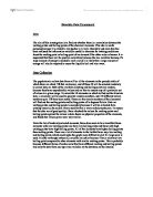
4-Day Division 1:
This graph showed me that, as my prediction had suggested, there was negative correlation within my data.
I took 24 results from the sample I took and this gave me my results.
When I tested this data to see if there was any correlation, I used the Pearson method to calculate the correlation gradient within my data. My results showed that:
The required gradient for correlation within the number of results I collected: -0.3438
The correlation my results concluded: -0.5984322355
This calculation shows us that because the correlation of my data falls within the required gap, there is correlation between the numbers of wickets taken by a Division 1 bowler compared to their bowling economy (Runs/Over).
As I saw that there was a correlation between The number of wickets taken by a Division 1 bowler compared to their bowling economy (Runs/Over), I decided to continue with my data collection and found data for the 2nd Division of the 4-Day competition, and both divisions of the 1-Day competition.
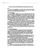
This is the graph that my results for the 2nd Division:
The required gradient for correlation within the number of results I collected: -0.3598
The correlation my results concluded: -0.253004785
We can see that this graph did not produce very good correlation but I will still conduct the correlation gradient test on it:
This calculation shows us that there is not enough correlation between the numbers of wickets taken by a Division 2 bowler compared to their bowling economy (Runs/Over) to create a correlation gradient. We can see this from my table:
These results show us that Division 1 bowlers are generally economic when they take more wickets than the Division 2 bowlers do.
I will now put both of these sets of results together to see if there is any general correlation between Division 1 and Division 2.
This is the scatter diagram is completed with the data:
The required gradient for correlation within the number of results I collected: -0.44566
The correlation my results concluded: -0.2455
We can see that this graph did not produce very good correlation but I will still conduct the correlation gradient test on it:
We can see that this confirms my prediction that there is not enough correlation to match the correlation gradient requirement.
I will now conduct the same results on the NUL 1-Day League.
NUL Division 1 (1 Day):
The required gradient for correlation within the number of results I collected: -0.3887
The correlation my results concluded: -0.425243392
This showed us that there was significant correlation within my results and I can prove this with this diagram:
This diagram shows that there is just significant correlation, and if I were going deeper into these results, I would conduct a 10% random test instead of the 5%, as I have been doing with all of my other results.
This is what the Division 2 scatter diagram looked like:
The required gradient for correlation within the number of results I collected: -0.3297
The correlation my results concluded: -0.643205772
This showed very good correlation and I can show this via this diagram:
This shows that there is definitely significant negative correlation within these results. My penultimate scatter diagram will be the complete 1-Day results:
The required gradient for correlation within the number of results I collected: -0.2483
The correlation my results concluded: -0.564624
This shows that overall; there was significant negative correlation within the 1-Day league.
We can see this for certain in this diagram:
My final scatter diagram will encompass all of my results, to see if there is any overall correlation:
The required gradient for correlation within the number of results I collected:
The correlation my results concluded: -0.5255
This shows that overall; there was significant negative correlation within all of my sample, and therefore my population.
Hypothesis Test
For all of my graphs, I have created a critical region table and showed on it, where my P.M.C.C value lie. However, I need a hypothesis to show this.
H0: no correlation; ρ = 0
H1: negative correlation; ρ < 0
This means that for each of my scatter diagrams, I am aiming to get significant negative correlation within my results (i.e. H1)
However, because the number of my results is greater than the final number in the P.M.C.C table, I will have to estimate my critical region. I do know that the correlation, which my graph has, exceeds the critical region for 60 statistics, so that shows me that my results will show significant positive correlation.
We can see that for my final scatter diagram that my required critical region is:
rcrit = < -0.2144
rtest = -0.5255
I can show these results in a graph:
Evaluation
Obviously, my results, and my correlation were not perfect but there will have been some results that were very peculiar. To remove these from my data I will use the technique of Standard Deviation.
To do this, I use the equation in EXCEL:
=STDEV (D2:D92)
This shows the equation itself (=STDEV), and the required field of my data (D2:D92).
Using this equation, we see that the standard deviation, for the economy of a bowler is:
1.216394
This means that any bowler whose economy is this far away from the median value (discovered in the Boxplots section) can be viewed as an insignificant piece of data.
This means that if we take all of the results from my final scatter diagram, we will be able to see which results are relevant.
I found out earlier in my coursework the median for my 4-Day players and 1-Day players. I will now find it for my complete results scatter diagram above, and this will enable me to find any outlying results. If I omit these results from the scatter diagram, I would get much better correlation.
All Statistics
(See attached sheet for box plot)
We can see from this chart that the Median is 4.14, and as we know that the Standard deviation for these results is 1.216394, we can see that any results less than 4.14 - 1.216394, or greater than 4.14 + 1.216394, can be considered as outliers. Therefore, we can see any “odd” results and highlight them as the cause of my correlation.
Overall this means that any results that are 2.923606 or below, or 5.356394 will be considered as outliers, and I can show a graph without any of these points in it now:
This graph gave me a correlation of:
-0.63308
This is much better than what I got for my original scatter diagram.
The Standard deviation technique has helped me to remove my “outliers” and complete a very successful Statistics coursework.
There are obviously ways in which I can improve my coursework, such as taking more results from a bigger sample. I could also do comparisons between a player’s international and domestic economy and wickets, to see whether players play better for their country.
These would create a deeper coursework. However, I do not have enough time to create this kind of coursework, so sadly I will have to settle with what I have.