My Hypothesis is that (in general), the taller the person is, the more they will weigh. To extend my investigation further, I will look at the height of girls and boys separately
Now, you can see from the above scatter diagram that there is definitely a clear relationship between height and weight and therefore, proves that my hypothesis (the taller the person is, the more they will weigh) is correct.
In order to organize the structure of my data in a simpler way I have put all of my data into frequency tables. I made 4 different tables each containing the frequency for boys and girls weights, and their heights.
Boys
Girls
I will then show these tally charts above onto four separate bar graphs each relating to boys/girls height and weight.
To make these graphs clearer to see, I will present the data in the form of two frequency polygon; one for girls and boys height, and one for girls and boys weight.
I can see from the frequency polygon that there are more girls with heights between 150 and 170cm than boys, but there are only a few more boys taller 170cm. This would suggest that possibly my hypothesis was not correct as there isn’t that much of a difference between boys and the girls.
This shows that the Boys’ data is more spread out than the girls. It also shows that there are fewer boys with weights between 20 and 60kg than girls. There are however more boys with weights higher than 60kg.
Averages for the data.
By looking at my frequency tables I will be able to determine what the mean, mode, median and range of all my data will be. From discovering these, I will be able to determine whether my hypothesises were correct. In order to find all these factors I will have to produce another frequency table.
To find the mode of the boys’ heights I will need to see which of my bars on my bar graph is the tallest. The group that is the tallest on my graph for boys’ height is 170 ≤ h < 180. Therefore the group: 170 ≤ h < 180 is where the modal number is.
To find out the mean, I have to add in three extra columns to my frequency charts. I have to obtain the midpoint of each of the values, of all the different ranges of heights. Then, i had to multiply the midpoint by the frequency. Once I had done this with every height range, I added the totals together. This would give me my ‘fx’ coloumn. I also added up the total amount of boys which was correctly 25 (showing no errors were made in the tally chart).
Therefore, the mean for the boys’ height is: x = ∑fx = 4195 = 167.8
∑f 25
The median for this data lies within the data is: 170 ≤ h < 180. This is because the 12th and 13th value lies between this range.
In order to find the range, I will take the highest boys height from the lowest height.
Therefore, we would take 1.92 (highest height) – 1.35 (lowest height) = 0.57m
To find the averages of boys’ weight and girls’ height and weight, I will follow the same order and processes which I used for the boys height.
The mode of this data is: 50 ≤ h < 60.
The mean for this data is: x = ∑fx = 1315 = 52.6
∑f 25
The median for this data lies within the data is: 50 ≤ h < 60
The range in boys weights: 69 – 29 = 40kg
The mode for this data is: 140 ≤ h < 150.
The mean for this date is : x = ∑fx = 3955 = 158.2
∑f 25
The median for this data is: 150 ≤ h < 160
The range in girls’ heights is : 1.83 – 1.42 = 0.41m
The mode of this data is: 40 ≤ h < 50.
The mean for this data is: x = ∑fx = 1125 = 45
∑f 25
The median for this data lies within the data is: 40 ≤ h < 50
The mean for this data is: x = ∑fx = 1315 = 52.6
∑f 25
The median for this data lies within the data is: 40 ≤ h < 50.
The range for girls’ weight is: 60 – 29 = 31
I have discovered that, after working out the mean of both the boys’ and girls heights and weights, that in fact the both the boys height and weights are higher than the girls’. This proves that my hypothesis is correct.