When looking at the aggregate demand curve we also have to look at the ISLM model, in particular the IS curve and how it is derived.
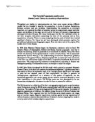
Looking at the graph below, if interest rates are at R, investment and saving is affected by it. National income equilibrium is where I = S. if the rate of interest changes from R to R1 then it will cause a rise in investment and a fall in savings. A rise in investment would cause a shift from I to I1 and a shift in saving from S to S1. In the lower part of the diagram
We can see from the graph that it gives rise a downward sloping I=S curve. This curve shows national income, which is another way of showing demand for the whole economy. The IS curve is relatively steep because the investment demand curve is relatively inelastic, due to unresponsiveness investment to changes in interest rates. Saving is also unresponsive to interest rate changes. Hence why the AD curve is sometimes shown as downward sloping.
Aggregate supply is the amount of total production for the nation for some period. Government is concerned about aggregate supply and the ability of ones economy to produce goods and services.
The aggregate supply curve shows the relationship between the level of total output of goods and services, (measured by real GNP), and the general level of prices in the economy. Due to inflation, prices will rise and total amount of output will change too. There is more than one shape of the AS curve, depending on the state of the national economy.
If an economy is in a depression or a recession there is a surplus of unemployed resources such as workers, factories and natural resources. Because there are so much highly productive resources that are not being used, firms that wish to expand will not have to bid up input prices in order to acquire the resources necessary to expand production.
Because of productive unemployed resources available at no increase to cost, it means that there will be a ‘depression’ aggregate supply curve shown below. The curve is horizontal, which shows that more output may be obtained without any affect on the price level.
Price Level
AS
GNP
The aggregate supply curve can also have another shape to it when it is in a full employment aggregate supply economy. It is just the opposite of the depression economy. In this situation all the economy’s resources are being used, so when ever a firm which to expand output, resources will be taken away from another firm. This causes factor prices such as wages and rent to rise. This results in vertical aggregate supply curve. It shows that in the short run there is maximum possible production in the economy and it is impossible to produce any more output. If a firm attempted to increase production it would lead to higher prices. This is because firms will have to offer more money to obtain machines etc. causing prices to rise in general.
This would cause the aggregate supply curve to be a perfectly vertical slope. Since all the resources are fully utilised, any attempts to increase output results only in rapid inflation.
Price Level AS
GNP
The two supply curves mentioned above are extremes of an economy. The more common type of economy is called a bottleneck Aggregate Supply economy. In this economy there is some substantial unemployment, but not as much as there would be in the depression economy. Most but not all resources are employed and working. This results in aggregate output only being increased with an increase in price level. Output can be expanded but the resulting bottlenecks and inefficiencies cause the price level to rise. Inflation must accompany increase in real GNP. This type of aggregate supply curve is a supply curve in the long run of an economy as it contains all three characteristics and the economy moves from one range to another as economic growth or decline takes place.
Price AS
GNP
In conclusion we can see that the AD and AS curve can take many forms of shape, but for all different reasons. These reasons are to do with the economy and what sort of financial position they are in.