Newton Raphson
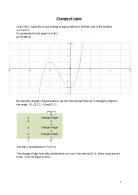
y=0.5x³+1.5x²–x–0.25
Example y=0.5x³+1.5x²–x–0.25
Graph of y=f(x) function
There are roots in the intervals [-4, -3], [-1, 0] and [0, 1].
I am going to find the root in interval [-4, -3].
By using the Newton Raphson method:
If
Then
Therefore,
To find the root between interval [-4, -3]
Let x1=-3
We can see that root is near to -3.5269 to 5 sf
Using Newton Raphson and Autograph to find the root in the interval [-4,-3]:
We now are using the Newton Raphson and Autograph to find the other two roots.
I can see that the other roots lie within these intervals [-1, 0] and [0, 1]:
From the table below, I can find out that the root in the interval of [-1, 0] is near to 0-3.5269 of 5 significant figures.
On the other hand, from the table below, I can find out that the root in the interval of [0, 1] is near to –0.19609 of 5 significant figures.
Graphical Interpretation of the Newton Raphson method
Example: y=2x y=0.5x³+1.5x²–x–0.25
Graph of y=f(x)
I will first use the method to find the root at the interval [-3, -4]
y=0.5x³+1.5x²–x–0.25
X2
X3
X4
X1
At first, let’s start with a close approximation, let X1= -3, on the x-axis (shown on the graph above), draw a verticle line until it meet y=0.5x³+1.5x²–x–0.25.
When the line met the curve, a tangent is drawn and extended until it meets the x-axis and there is a new point on the x-axis, called X2, which is equal to -3.7858.
From X2, draw a vertical line until it meet the curve y=f(x). When the line met the curve, a tangent is drawn and extended until it meets the x-axis and it is a new point on the x-axis, called X3, which is equal to -3.5566.
From X3, draw a vertical line until it meet the curve y=f(x). When the line met the curve, a tangent is drawn and extended until it meets the x-axis and it is a new point on the x-axis, called X4, which is equal to -3.5273.
This procedure is repeated and the points generated on the x axis get nearer and nearer to the root.
At last, I can see that Newton Raphson converges to a value near to -3.5269.
Error Bounds
We need to use the change of sign method to trap the root between two solution bounds
I evaluate f(-3.52695) and f(-3.52685):
f(-3.52685)=-0.00051
f(-3.52695)=0.000193
This change of sign shows that the root must be between these two values. Therefore,
I can state that the error bounds are -3.52695 and -3.52685
I can also write the solution bounds as the error bounds-3.5269±0.00005
I can see that all values in the range (-3.52685, -3.52695) round to -3.5269. Therefore, I can say that the root is -3.5269to 5 sig.figs.
Failure Case
Example: y= (0.5x³+1.5x²–x–0.25) 1/3
Reason cause to failure is that the graph crosses the x axis with a very steep gradient
Graph is y=f(x)
The steep crossing points were caused by the power 1/3
On the graph, the Newton Raphson method will fail to reach a root
y= (0.5x³+1.5x²–x–0.25) 1/3
X3
X2
X1
Newton Raphson method does not work everytime. Newton Raphson method will fail when I consider operating the process on the function f(x) = x1/3, start with the initial value x=-3.
As you can see, from the start point of -3, the values of Xn become further and further away from the root between -3.52695 and -3.52685. This is because of the steep gradient where the graph crosses the x-axis, meaning that the resulting tangent is directed further away from the root.
x=g(x) method
y=0.8x³+2x²–x–1
I am now using the example y=0.8x³+2x²–x–1 to illustrate the method of x=g(x).
Graph of y=f(x) function
Now, rearrangement of the equation f(x) =0 to the form x = g(x)
I have got the function y=0.8x³+2x²–x–1,
Therefore, 0.8x³+2x²–x–1= 0
0.8x³= -2x²+x+1
At last, I can see that
Use the example 0.8x³+2x²–x–1= 0 and find the root in the interval [-3, -2], let X1 = -3,
By using x=g(x), I can find the root in the interval [-3,-2]
From the table above, I can see that root is near to -2.7876 to 5 sf
Illustrating the convergence using x = g(x) by using Autograph.
y= x
X1
X2
X3
X4
X5
y=
First of all, we can see that the root is near -1, so start at a point x1 , which is -1, on the x axis line and draw a line vertically downwards to meet the curve y=f(x).
When the line meets the curve y= f(x), a horizontal line is drawn to meet the line y= x.
The x co-ordinate of this new point becomes x2
From x2, we draw a line vertically downwards until it meet the curve y= f(x) again. And a horizontal line is drawn and meet the straight line y=x.
The x co-ordinate of this new point becomes x3
These steps will repeat and new points are generated nearer and nearer to the point of interception of y=x and y=g(x) which is the root of equation of f(x) =0
Examining g’(x) graphically
y=x so gradient 1
We can see 0<g’(x)<1
Root to f(x) =0
Since 0<g’(x)< 1 we expect to get staircase convergence and it is a success staircase and the result is the same as the expectations.
A rearrangement of the same equation is applied in a situation where the iteration fails to converge to the required root
Roots are given by 0.8x³+2x²–x–1= 0,
Then, make a new rearrangement of the function f(x)= 0 to the form x = g(x)
0.8x³+2x²–x–1= 0
Then x= 0.8x³+2x²–1
xn+1= 0.8xn3+2 xn2-1
To find root in the interval [0, -1]
Let X1=0,
From the table above, we can see that the iteration is diverging away from the root in interval [0, -1]
This is illustrated graphically below:
X3
y= 0.8x³+2x²-x–1
X1
y= x
X2
We can conclude that g'(x) < -1 then the iteration will diverge away from the root in a cobweb fashion and it will become a failure case
Evaluating g'(x) using calculus
Since g(x) = 0.8x³+2x²–1
g'(x) = 2.4x2+4x
The roots were x = -2.7876 ([-3, -2]) or -0.54113([-1, 0]) or 0.82868([0, 1]).
Hence g‘(root) in the interval [0, 1]= -1.4617
As g’(x) < -1, we can expect that the iteration to diverge away from the root in a cobweb fashion. This can be shown on the graph above, and therefore this must be correct.
Comparisons
Now, I am going to compare all the 3 methods I have used in the coursework, including change of signs method, Newton Raphson method and x=g(x) method. In order to do so, I will first use the equation which was used in change of signs, x³+3x²–3=0, and use the Newton Raphson method and x=g(x) method to find the same roots.
y= x³+3x²–3
By using Decimal search:
Find the root in the interval [0, 1],
Secondly, I will use Newton Raphson method to find the same root in the interval [0, 1]:
First of all, I need to rearrange the equation x³+3x²–3=0 to the formulae of Newton Raphson (
)
Then
Find the root between interval [0, 1],
Let X1 be 1,
The root is 0.87939±0.000005
f(0.879385) = 0.879385241
f(0.879395) = 0.879385241
The root is trapped between 0.879385 and 0.879395.
Therefore, the root is 0.87939 to 5 decimal places.
Lastly, we will use x=g(x) method to find the root in the interval [0, 1]:
I need to rearrange the equation x³+3x²–3=0 in to the form of x=g(x),
Let X1= 1
x³+3x²–3=0
f(0.879385) = 0.879385241 and f(0.879395) = 0.879385241
The root is trapped between 0.879385 and 0.879395
We can see that the root is 0.879385± 0.000005 or 0.87939 to 5 decimal places.
Comparisons among all three methods
From the table above, it shows there are 36 calculations for change of signs, 5 calculations for Newton Raphson and 18 calculations for x=g(x). To conclude, Newton Raphson method is the quickest in find the root, followed by x=g(x) method and the slowest is change of signs method.
Relative merits of the three methods with available hardware and software
If you only had a scientific calculator
During the ways finding the roots, we know that by using scientific calculator, we are able to look for the roots by all methods. If I only had a scientific calculator, Newton Raphson will be the fastest way to find the roots. The reason is that it only involves a few calculations and it is easy to calculate them.
On the other hand, change of signs method involves a number of tables and it makes it inconvenience for us to find the roots. Also, if the too roots are too close together, we might miss the other two after finding the first one. Consequently, we would be unlikely to seach further in the intervals.
Despite the fact that x=g(x) method also involved some calculations, it’s not the quickest way to find all the roots and therefore, Newton Raphson is the best method to solve the equation.
If you only had a graphic calculator
By using graphic calculator, we can draw the graph out first, which may let us see if there is going to be a clear change of sign. If so, I think that the decimal search will be the simplest way to find the roots. Also, using change of signs method with graphic can guarantee that the method should be worked; it seems it takes a bit longer than other methods, though. What is more? There is a function of zooming in the graph in the graphic calculator, which makes it easier to find out the values that correct to 5 decimal places.
Nevertheless, if we cannot see there is going to be a clear change of signs, Newton Raphson method would probably the quickest method among three of them, though it may be a bit complicated.
If you also have Excel
All these methods can be carrying out simply by using the spreadsheet such as Excel. But among the three methods, I think change of signs method should be chosen as the easiest and quickest one. There isn’t any iteration and rearrangement involved in the formulae and it is very easy to enter all the information into Excel.
Whereas we need to rearrange the formulae for Newton Raphson method and x=g(x) method, which we may enter the wrong figure into Excel by mistake and it is really complicated.
If you also have Autograph
Obviously, we can find the roots in no time by using Autograph. For change of signs method, we simply draw a graph by using Autograph and find the roots when f(x) = 0. It’s very easy for us to use autograph and it just involves one step. After finding the roots, we can leave Autograph and use Excel to proof the rest of the change of signs method.
For other two methods, we need to do more steps. For example, we need to set up another equation y=x in x=g(x) so that we can continue to do the rest of the x=g(x) method.