I understand that this sample eradicates all other cars from the list and other types of car may not be affected in the same way as 1.4 engined cars.
HYPOTHESIS 2
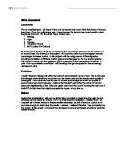
“Cars with short MoTs are frequently sold.”
In order to test this I am going to draw a cumulative frequency diagram. I have decided to use cumulative frequency so that I can find the interquartile range of the months of MoT left. This will show me the average amount of MoT left when cars, in my sample, are put up for sale.
On my diagram I will have 5 distributions so that I have a good range of data to show on my diagram. (Appendix 3)
This graph shows that the average time left is between 2 and 9 months. The results of this may be wrong as there are 3 cars in my sample that do not have to have an MoT as they are less than 3 years old.
HYPOTHESIS 3
“Most cars within my sample will have done between 50,000 and 60,000 miles.”
I will draw a frequency polygon to prove this. (Appendix 4)
I am going to use a frequency polygon for this, so that I can group my data in to six different groups and use the average mileage within each group to show in the graph.
There are only 20 cars in this table, as the VW Golf, car no. 29, does not have a mileage shown. That is an anomalous result.
I discovered that most of the cars had done an average of 30,000 miles. This proves my hypothesis wrong, as it was about half of my prediction.
HYPOTHESIS 4
“The estimated mode for car manufacturers in my sample is Ford.”
I will use a tally chart to record my results.
Again, my hypothesis was proved wrong, as Vauxhall is the most frequently sold second hand car along with VW.
HYPOTHESIS 5
“Make and age of car will influence price”
I will now calculate the mean average second hand cost of Vauxhall and VW cars in this sample to see whether they have similar prices. I am only using these two makes of car as they are the modal makes of car in my sample.
(figures in £ sterling)
VW
400 + 3695 + 7550 + 4693 = 16338 / 4 = 4084.50
Vauxhall
7499 + 1000 + 4976 + 3191 = 16666 / 4 = 4166.50
There is a very strong link between the prices for these two makes of car since the price difference is only £82. This suggests that the make of middle range cars does not affect prices of second hand cars. However, we do have one extreme in the VW of £400.
I will now investigate the average of these cars to see if there is any link between price and the age at which they are sold.
VW
15 + 7 + 1 + 5 = 28 / 4 = 7
Vauxhall
4 + 10 + 4 + 6 = 24 / = 6
So, I can come to the conclusion that 1 year’s difference between these two cars average makes £82 difference in price. This is a small difference, but again the low price and high age of one of the VW cars could be distorting the results. This proves my hypothesis to be incorrect as price does not seem to be affected as much as I would have expected.
HYPOTHESIS 6
“Random cars selected at random will be red.”
In order to test this I am going to use a tally chart and then calculate the probability of this statement being true.
I have used this information to draw a pie chart, showing the % within my sample of each colour car (appendix 5)
This shows my hypothesis to be correct, as there is a probability of 0.43 of the second hand car being red. This means that if I randomly selected any number of cars there is a 43% chance of it being red.
I am now going to find out the median tax group (just because I want the marks!)
0 1 2 3 3 3 3 3 4 4 4 4 5 5 5 5 6 8 9 9 12
The median is 4.
The estimated probability of the length of tax left on the car affecting the price of cars is 20%.
I have drawn a histogram (appendix 6) showing the frequency of prices of second hand cars in my 1.4 engine sample. This shows that the highest frequency is for cars that cost between £4,000 and £4,999. The peculiarity of this result is that in the £5,000 - £5,999 and £6,000 - £6,999 price bands that follow the mode, have no frequency. Also in the £9,000 - £9,999 price band there is no frequency but this has price bands either side of it that have a frequency of 1. This may mean that the sample is too small to draw a statistically reliable conclusion.
CONCLUSIONS
I was asked to investigate what influence the prices of second hand cars. My first hypothesis was that the age of the car would affect prices. There was a strong positive correlation between depreciation and price showing that older cars will be cheaper than newer ones.
My second hypothesis was that cars with short MoTs are frequently sold. The cumulative frequency showed the interquartile range to be between 2 and 9 months left on the MoT. It was difficult to interpret the results on this as 3 cars in the sample did not have to have MoTs as they were under 3 years old. This makes the data unreliable so I cannot draw a reliable conclusion for this hypothesis.
My third hypothesis concerned mileage. I was surprised to find that second hand cars are most likely to have only a mileage of 30,000.
My fourth hypothesis showed that Vauxhall is the most frequently available second hand car.
Hypothesis 5 looked to see if make and age of car would influence price. I found that the make of car did not seem to influence the second hand value as strongly as I would have thought. There was a strong correlation between these sets of data.
Hypothesis 6 suggested that cars, selected at random, there was a 0.43 probability of this being true. This is a strong correlation when considering all the different colours of car available.
It is likely that a buyer will want about 4 months of tax on a second hand car.
Whilst there were some strong correlations, particularly that between age of car and price, the histogram showed that my sample might be too small to predict the true influences on prices of second hand cars.