I will test them for any relation they may have and draw scatter diagrams.
The scatter diagrams would have lines of best fit.
A cumulative frequency table may also be useful in finding the relations.
The information I need to collect are the prices and the mileage. These are available in the excel spreadsheet from the KGV math site and I will be working form this. The spread sheet is reliable as it is provided for us. It contains a sample of 100 cars.
I will take three samples of 10 using stratified sampling (taking a few from each 10) and leaving out the extremes from both ends. This will give a fair sample as all the different percentages are taken into account.
The samples will be compared to each other to find if there is a correlation.
I will also find the correlation coefficient using the formulas:
∑ x;y - ∑x; ∑y ∑ x2 – (∑x;)2 ∑y;2 - (∑y;) 2
n n n
Prediction
I think that there will be a strong positive correlation as usually, the price drops by a greater percentage as the mileage increases.
Hypothesis
I think that this will be true as older cars get sold for less money. This is generally what happens but in some circumstances, for example, a 7 year old Rolls Royce that has traveled 100000 miles can cost more that a brand new Toyota.
Results
The pretest graph:
This showed that the data has strong positive correlation and would be worth investigating into.
The correlation coefficient of the original sample was: 0.9865 this figure is very close to 1.00 and so, this also proves that the sample has a very strong positive correlation.
The cumulative frequency table allows me to work out the divination by the formula:
n∑x2 –(∑x)2 = 38.71366
n2
The cumulative frequency curve shows that most cars have dropped between 20 and 40 percent from their original price and at that point, their mileage would have been from 24000 t o 50000.
Here are the correlation coefficients for all my three samples:
Sample 1: 0.989297 Sample 2: 0.989546 Sample 3 : 0.990238
All the scatter diagrams show a strong positive correlation as their points nearly make a straight line.
Conclusion
From the results, I have made the following observations:
Using a scatter diagram, I found that there is a strong positive correlation between the percentage decrease and mileage
·With either of X or Y, I could estimate the other with the line of best fit.
The cumulative frequency tells me that most cars decrease between 20 and 40 percent in price.
Evaluation
The investigation could have been brought to a greater extent if more strategies have been used to analyze the data such as box and whiskers diagrams or histograms at the start of the coursework.
The observations were as predicted and the results were acceptable.