Theory:
Simple Harmonic Motion (SHM) is the regular movement of an object about a central point. The acceleration is always in the direction towards the central point. If the displacement of the object from the central point is X then the acceleration to the centre is proportional to X.
So, using this diagram, my theory goes as follows:
When the weight is below the EP, Hooke’s Law provides a force pulling upwards equal to KX. When the weight is above the EP the balance of the Gravitational Force (from Hooke’s Law) equals a force KX pulling down towards the EP.
So the force pulling towards the EP equals KX, where K = spring constant. As F = ma, the acceleration is (K/m)X against the motion and we have simple harmonic motion.
Given this information, we can work out the time period for an oscillation under these circumstances: T = 2∏√ (m/K). So, if T=2∏√(m/K), also written as T² = (4∏²/K²)m, then T √m.
This should be correct, only while Hooke’s law applies, and will only happen when the extension, X, is less than the value of L. Note: The value of T is independent of the original extension.
Prediction:
My prediction is that the more weight that is added to the bottom of the spring, the more energy is stored, and therefore will create larger oscillations. This is because according to my theory (above), the heavier the mass put on the spring, the larger the extension will be. So, if this is correct, there will be more energy, therefore resulting in larger oscillations.
In a graph, according to my theory, if T is plotted against m, the results should be shown as below (left) or if T² is plotted against m the results should be shown as below (right):
Factors:
In this investigation, there are three main factors to consider. These are
(a) – The size of the spring - Three different springs were tested in the preliminary experiment, and proved that different sizes have different results even with the same equipment being used as each spring has its own individual limits.
(b) – The mass on the spring – Several different masses were put on the springs in preliminary tests and showed that the wider the mass range, the wider the range of oscillation times was.
(c) – How far the spring is pulled down – The distance from when the spring is in equilibrium to where it is stretched to, to start oscillating from, affects the steadiness of the spring. This was also tested in the preliminary experiment and showed that the longer the distance, the less steady the spring became and the more likely it was to swing than to oscillate straight down vertically.
Precautions:
The safety precautions I have taken into account are as follows:
(a) – Don’t pull the spring too far down, as this could result in the masses falling off and could hurt someone.
(b) – Make sure the stand is stable and secure on the table, as if it isn’t, it could fall and hurt someone.
(c) – Make sure the spring is secured properly to the clamp, as if it isn’t, it could again, send heavy weights flying off.
So as not to interfere with actual experiment, the precautions that I have taken into account and amended from the preliminary experiment are as follows:
- – The spring’s elastic limit – The spring cannot be overstretched for two reasons. These are:
I - If it is pulled too far, the oscillations would be uneven, unsteady and would be difficult to record, and
II – If the spring goes past its elastic limit, it wouldn’t work properly and would eventually be just a piece or wire.
(b) – The way the spring is attached to the clamp – This is important because lalalal if the spring is not self-suspended, it could affect the size, number, and lallala speed of each individual oscillation.
Results:
First Set Of Results
Second Set Of Results
Third Set Of Results
Average Set Of Results
The results highlighted in red, are those that I have recorded as anomalous, as they do not act in accordance with the theory. Looking at each of my graphs, there is a curve in each. In most of them, the line changes to a curve at 500g.
Analysis II:
From my T² graph and the equation, 4∏²/K²=gradient we can find out the constant, K by finding the gradient of the line.
Gradient: (900, 1.08)
(200, 0.25) = 0.83/700
So, 4∏²/K² = 083/700
4∏² x 700 = 0.83 x K²
2800∏²/0.83 = K²
√ (2800∏²/0.83) = K
K = 182 (3.s.f.)
Conclusion:
‘T’ against ‘m’
I would say that my prediction graph does not fully resemble the average graph that I have produced from my results. The red line on this graph is the line showing my actual results, and the black line is my line of best fit. The black line, however, leaves too many anomalous results and I feel that a curve of best fit might have been appropriate in this case. This is because my red line is as such of two lines which bend in the middle giving the impression of a curve. Therefore, my prediction graph was correct in shape, but my actual graph was only partially correct.
‘T²’ against ‘m’
I would say that my prediction graph does resemble the average graph that I have produced from my results. Again, the red line shows my actual results and the black line shows my line of best fit. This time however, the line of best fit proves that T² is directly proportional to m as it is a straight line graph. Therefore proving my prediction was in fact correct.
Evaluation:
Overall, I think my experiment was carried out quite well, and I managed to get fairly accurate results too. I do however think that I could’ve done better in several ways.
The first thing I would change about the way in which I did my experiment would be to carry out more preliminary tests. For one, this would increase the way in which I carried out my experiment, and two, this would give me more information on the spring that I could use. For example if I had tested to see if there was an effect on the oscillations if the spring was displaced upwards instead of down to begin with.
The second is by increasing the number of recordings taken. In doing this, my experiment would’ve been more accurate due to the fact that I’d have more results to look at.
The next thing I could’ve done was to use 50g weights instead of 100g. This would also improve my results as they would be closer together and it would be easier to point out any anomalies that may have occurred.
The last thing I could’ve done would be to amend my graphs. So, instead of drawing a line of best fit, I could’ve drawn a curve of best fit instead, seeing as the graph itself was in the shape of a curve. Not only would this have been easier to look at and analyse, but it would reduce the number of anomalies created.


